Power Plots in statsmodels

I just want to show another two plots for the statistical power of a test, since I didn't have time for this earlier

The code to produce them is just calling the methods of the power classes, for example for the one sample t-test.

Help: I caught a bug

I think I must be turning too much into a statistician and econometrician lately, I must have caught a virus or something. Maybe it started already a while ago

The theme of the scipy conference this year is "Machine Learning & Tools for Reproducible Science". However, I'm not doing any sexy twitter analysis, I just spent some days coding tests for proportion, boring stuff like pairwise comparisons of proportions.

Anyway, I decided to submit a tutorial proposal for econometrics with statsmodels to the scipy conference, see (lightly edited) proposal below. Since my proposal didn't get accepted, my first response was: Wrong topic, Too much statistic, We just want numbers, not check whether the model is correct, and find out how to fix it.

That leaves me with more time to go back to figuring out which other basic statistical tests are still missing in Python.

Statistics in Python: Reproducing Research

This is just a short comment on a blog post.

Ferando Perez wrote a nice article about "Literate computing" and computational reproducibility: IPython in the age of data-driven journalism

In the second part, he explains that Vincent Arel-Bundock came up with an ipython notebook within three hours to replicate some criticism of an economics journal article. Vincent's notebook can be seen here.

What I found most striking was not the presentation as a notebook, although that makes it easy to read, instead it was: pandas, patsy and statsmodels, and no R in sight. We have come a long way with Statistics in Python since I started to get involved in it five years ago.

Vincent has made many improvements and contributions to statsmodels in the last year.

Aside

I'm not following much of the economics debates these days, so I only know what I read in the two references that Fernando gave.

My impression is that it's just the usual (mis)use of economics research results. Politicians like the numbers that give them ammunition for their position. As economist, you are either very careful about how to present the results, or you join the political game (I worked for several years in an agricultural department of a small country). (An example for the use of economics results in another area, blaming the financial crisis on the work on copulas.)

"Believable" research: If your results sound too good or too interesting to be true, maybe they are not, and you better check your calculations. Although mistakes are not uncommon, the business as usual part is that the results are often very sensitive to assumptions, and it takes time to figure out what results are robust. I have seen enough economic debates where there never was a clear answer that convinced more than half of all economists. A long time ago, when the Asian Tigers where still tigers, one question was: Did they grow because of or in spite of government intervention?

Multiple Testing P-Value Corrections in Statsmodels

series : "Statistics in Python"

This is a follow-up to my previous posts, here and this post, which are on software development, and multiple comparisons which looks at a specific case of pairwise mean comparisons.

In the following, I provide a brief introduction to the statsmodels functions for p-value asjustements to correct for multiple testing problems and then illustrate some properties using several Monte Carlo experiments.

Debugging: Multiple Testing P-Value Corrections in Statsmodels

subtitle: "The earth is round after all"

series : "Adventures with Statistics in Python"

If you run an experiment and it shows that the earth is not round, then you better check your experiment, your instrument, and don't forget to look up the definition of "round"

Statsmodels has 11 methods for correcting p-values to take account of multiple testing (or it will have after I merge my latest changes).

The following mainly describes how it took me some time to figure out what the interpretation of the results of a Monte Carlo run is. I wrote the Monte Carlo to verify that the multiple testing p-value corrections make sense. I will provide some additional explanations of the multiple testing function in statsmodels in a follow-up post.

Let's start with the earth that doesn't look round.

experiment:

Monte Carlo with 5000 or 10000 replications, to see how well the p-value corrections are doing. We have 30 p-values from hypothesis tests, for 10 of those the null hypothesis is false.

instrument:

statsmodels.stats.multipletests to make the p-value correction

The first results

==========================================================================================
         b      s      sh     hs     h    hommel  fdr_i  fdr_n  fdr_tsbky fdr_tsbh fdr_gbs
------------------------------------------------------------------------------------------
reject 9.6118 9.619  9.7178 9.7274 9.7178  9.72  10.3128 9.8724  10.5152  10.5474  10.5328
r_>k   0.0236 0.0246 0.0374 0.0384 0.0374 0.0376  0.2908 0.0736   0.3962   0.4118   0.4022
------------------------------------------------------------------------------------------

The headers are shortcuts for the p-value correction method. In the first line, reject, are the average number of rejections across Monte Carlo iterations. The second line, r_>k, are the fraction of cases where we reject more than 10 hypothesis. The average number of rejections is large because the alternative in the simulation is far away from the null hypothesis, and the corresponding p-values are small. So all methods are able to reject most of the false hypotheses.

The last three methods estimate, as part of the algorithm, the number of null hypotheses that are correct. All three of those methods reject a true null hypothesis in roughly 40% of all cases. All methods are supposed to limit the false discovery rate (FDR) to alpha which is 5% in this simulations. I expected the fraction in the last line to be below 0.05. So what's wrong?

It looks obvious, after the fact, but it had me puzzled for 3 days.

Changing the experiment: The above data are based on p-values that are the outcome of 30 independent t-tests, which is already my second version for generating random p-values. For my third version, I changed to a data generating process similar to Benjamini, Krieger and Yekutieli 2006, which is the article on which fdr_tsbky is based. None of the changes makes a qualitative difference to the results.

Checking the instrument: All p-values corrections except fdr_tsbky and fdr_gbs are tested against R. For the case at hand, the p-values for fdr_tsbh are tested against R's multtest package. However, the first step is a discrete estimate (number of true null hypothesis) and since it is discrete, the tests will not find differences that show up only in borderline cases. I checked a few more cases which also verify against R. Also, most methods have a double implementation, separately for the p-value correction and for the rejection boolean. Since they all give identical or similar answers, I start to doubt that there is a problem with the instrument.

Is the earth really round? I try to read through the proof that these adaptive methods limit the FDR to alpha, to see if I missed some assumptions, but give up quickly. These are famous authors, and papers that have long been accepted and been widely used. I also don't find any assumption besides independence of the p-values, which I have in my Monte Carlo. However, looking a bit more closely at the proofs shows that I don't really understand FDR. When I implemented these functions, I focused on the algorithms and only skimmed the interpretation.

What is the False Discovery Rate? Got it. I should not rely on vague memories of definitions that I read two years ago. What I was looking at, is not the FDR.

One of my new results (with a different data generating process in the Monte Carlo, but still 10 out of 30 hypotheses are false)

==============================================================================================
              b      s      sh     hs     h    hommel fdr_i  fdr_n  fdr_tsbky fdr_tsbh fdr_gbs
----------------------------------------------------------------------------------------------
reject      5.2924 5.3264 5.5316 5.5576 5.5272 5.5818 8.1904 5.8318   8.5982   8.692    8.633
rejecta     5.2596 5.2926 5.492  5.5176 5.488  5.5408 7.876  5.7744   8.162     8.23    8.1804
reject0     0.0328 0.0338 0.0396  0.04  0.0392 0.041  0.3144 0.0574   0.4362   0.462    0.4526
r_>k        0.0002 0.0002 0.0006 0.0006 0.0006 0.0006 0.0636 0.0016   0.1224   0.1344   0.1308
fdr         0.0057 0.0058 0.0065 0.0065 0.0064 0.0067 0.0336 0.0081   0.0438   0.046    0.0451
----------------------------------------------------------------------------------------------

reject : average number of rejections

rejecta : average number of rejections for cases where null hypotheses is false (10)

rejecta : average number of rejections for cases where null hypotheses is true (20)

r_>k : fraction of Monte Carlo iterations where we reject more than 10 hypotheses

fdr : average of the fraction of rejections when null is true out of all rejections

The last numbers look much better, the numbers are below alpha=0.05 as required, including the fdr for the last three methods.

"Consider the problem of testing m null hypotheses h1, ..., hm simultaneously, of which m0 are true nulls. The proportion of true null hypotheses is denoted by mu0 = m0/m. Benjamini and Hochberg(1995) used R and V to denote, respectively, the total number of rejections and the number of false rejections, and this notation has persisted in the literature. <...> The FDR was loosely defined by Benjamini and Hochberg(1995) as E(V/R) where V/R is interpreted as zero if R = 0." Benjamini, Krieger and Yekutieli 2006, page 2127

Some additional explanations are in this Wikipedia page

What I had in mind when I wrote the code for my Monte Carlo results, was the family wise error rate, FWER,

"The FWER is the probability of making even one type I error in the family, FWER = Pr(V >= 1)" Wikipedia

Although, I did not look up that definition either. What I actually used, is Pr(R > k) where k is the number of false hypothesis in the data generating process. Although, I had chosen my initial cases so Pr(R > k) is close to Pr(V > 0).

In the follow-up post I will go over the new Monte Carlo results, which now look all pretty good.

Reference

Benjamini, Yoav, Abba M. Krieger, and Daniel Yekutieli. 2006. “Adaptive Linear Step-up Procedures That Control the False Discovery Rate.” Biometrika 93 (3) (September 1): 491–507. doi:10.1093/biomet/93.3.491.

Inter-rater Reliability, Cohen's Kappa and Surprises with R

Introduction

This is part three in adventures with statsmodels.stats, after power and multicomparison.

This time it is about Cohen's Kappa, a measure of inter-rater agreement or reliability. Suppose we have two raters that each assigns the same subjects or objects to one of a fixed number of categories. The question then is: How well do the raters agree in their assignments? Kappa provides a measure of association, the largest possible value is one, the smallest is minus 1, and it has a corresponding statistical test for the hypothesis that agreement is only by chance. Cohen's kappa and similar measures have widespread use, among other fields, in medical or biostatistic. In one class of applications, raters are doctors, subjects are patients and the categories are medical diagnosis. Cohen's Kappa provides a measure how well the two sets of diagnoses agree, and a hypothesis test whether the agreement is purely random.

For more background see this Wikipedia page which was the starting point for my code.

Most of the following focuses on weighted kappa, and the interpretation of different weighting schemes. In the last part, I add some comments about R, which provided me with several hours of debugging, since I'm essentially an R newbie and have not yet figured out some of it's "funny" behavior.

Multiple Comparison and Tukey HSD or why statsmodels is awful

Introduction

Statistical tests are often grouped into one-sample, two-sample and k-sample tests, depending on how many samples are involved in the test. In k-sample tests the usual Null hypothesis is that a statistic, for example the mean as in a one-way ANOVA, or the distribution in goodness-of-fit tests, is the same in all groups or samples. The common test is the joint test that all samples have the same value, against the alternative that at least one sample or group has a different value.

However, often we are not just interested in the joint hypothesis if all samples are the same, but we would also like to know for which pairs of samples the hypothesis of equal values is rejected. In this case we conduct several tests at the same time, one test for each pair of samples.

This results, as a consequence, in a multiple testing problem and we should correct our test distribution or p-values to account for this.

I mentioned some of the one- and two sample test in statsmodels before. Today, I just want to look at pairwise comparison of means. We have k samples and we want to test for each pair whether the mean is the same, or not.

Instead of adding more explanations here, I just want to point to R tutorial and also the brief description on Wikipedia. A search for "Tukey HSD" or multiple comparison on the internet will find many tutorials and explanations.

The following are examples in statsmodels and R interspersed with a few explanatory comments.

Statistical Power in Statsmodels

I merged last week a branch of mine into statsmodels that contains large parts of basic power calculations and some effect size calculations. The documentation is in this section . Some parts are still missing but I thought I have worked enough on this for a while.

(Adding the power calculation for a new test now takes approximately: 3 lines of real code, 200 lines of wrapping it with mostly boiler plate and docstrings, and 30 to 100 lines of tests.)

The first part contains some information on the implementation. In the second part, I compare the calls to the function in the R pwr package to the calls in my (statsmodels') version.

I am comparing it to the pwr package because I ended up writing almost all unit tests against it. The initial development was based on the SAS manual, I used the explanations on the G-Power website for F-tests, and some parts were initially written based on articles that I read. However, during testing I adjusted the options (and fixed bugs), so I was able to match the results to pwr, and I think pwr has just the right level of abstraction and easiness of use, that I ended up with code that is pretty close to it.

If you just want to see the examples, skip to the second part.

TOST: statistically significant difference and equivalence

or "Look I found a dime"

The Story

Suppose we have two strategies (treatments) for making money. We want to test whether there is difference in the payoffs that we get with the two strategies. Assume that we are confident enough to rely on t tests, that is, means are approximately normally distributed. For some reasons, like transaction cost or cost differences, we don't care about the difference in the strategies if the difference is less than 50 cents.
To have an example we can simulate two samples, and let's take as a true difference a dime, 0.1

payoff_s1 = sigma * np.random.randn(nobs)
payoff_s2 = 0.1 + sigma * np.random.randn(nobs)

I picked sigma=0.5 to get good numbers for the story.

Two Tests: t-test and TOST

We compare two test, a standard t test for independent samples and a test for equivalence, two one-sided tests, TOST:

stats.ttest_ind(payoff_s1, payoff_s2)
smws.tost_ind(payoff_s1, payoff_s2, -0.5, 0.5, usevar='pooled')

The null hypothesis for the t-test is that the two samples have the same mean. If the p-value of the t-test is below, say 0.05, we reject the hypothesis that the two means are the same. If the p-value is above 0.05, then we don't have enough evidence to reject the null hypothesis. This can also happen when the power of the test is not high enough given our sample size.
As the sample size increases, we have more information and the test becomes more powerful.
If the true means are different, then in large samples we will always reject the null hypothesis of equal means. (As the number of observations goes to infinity the probability of rejection goes to one if the means are different.)
The second test, TOST, has as null hypothesis that the difference is outside an interval. In the symmetric case, this means that the absolute difference is at least as large as a given threshold. If the p-value is below 0.05, then we reject the null hypothesis that the two means differ more than the threshold. If the p-value is above 0.05, we have insufficient evidence to reject the hypothesis that the two means differ enough.
Note that the null hypothesis of t-test and of TOST are reversed, rejection means significant difference in t-test and significant equivalence in TOST.

The Results

Looking at the simulated results:
small sample size:

nobs: 10 diff in means: -0.14039151695
ttest: 0.606109617438 not different    tost: 0.0977715582206 different

With 10 observations the information is not enough to reject the null hypothesis in either test. The t-test says we cannot reject that they are different. The TOST test says we cannot reject that they are the same.
medium sample size:

nobs: 100 diff in means: 0.131634043864
ttest: 0.0757146249227 not different    tost: 6.39909387346e-07 not different

The t-test does not reject that they are the same at a significance size of 0.05. The TOST test now rejects the hypothesis that there is a large (at least 0.5) difference.
large sample size:

nobs: 1000 diff in means: 0.107020981612
ttest: 1.51161249802e-06 different        tost: 1.23092818968e-65 not different

Both tests no reject their null hypothesis. The t-test rejects that the means are the same. However the mean is only 0.1, so the statistically significant difference is not large enough that we really care. Statistical significance doesn't mean it's also an important difference. The TOST test strongly rejects that there is a difference of at least 0.5, indicating that given our threshold of 0.5, the two strategies are the same.

The Script

import numpy as np
from scipy import stats
import statsmodels.stats.weightstats as smws

nobs_all = [10, 100, 1000]
sigma = 0.5

seed = 628561  #chosen to produce nice result in small sample
print seed
for nobs in nobs_all:
    np.random.seed(seed)
    payoff_s1 = sigma * np.random.randn(nobs)
    payoff_s2 = 0.1 + sigma * np.random.randn(nobs)

    p1 = stats.ttest_ind(payoff_s1, payoff_s2)[1]
    p2 = smws.tost_ind(payoff_s1, payoff_s2, -0.5, 0.5, usevar='pooled')[0]

    print 'nobs:', nobs, 'diff in means:', payoff_s2.mean() - payoff_s1.mean()
    print 'ttest:', p1,    ['not different', 'different    '][p1 < 0.05],
    print '   tost:', p2, ['different    ', 'not different'][p2 < 0.05]

Notes

Implementation:
The t-tests are available in scipy.stats. I wrote the first version for paired sample TOST just based on a scipy.stats ttest https://gist.github.com/3900314 . My new versions including tost_ind will soon come to statsmodels.
Editorial note:
I looked at tests for equivalence like TOST a while ago in response to some discussion on the scipy-user mailing list about statistical significance. This time I mainly coded, and spend some time looking at how to verify my code against SAS and R. Finding references and quotes is left to the reader or to another time. There are some controversies around TOST and some problems with it, but from all I saw, it's still the most widely accepted approach and is recommended by the US goverment for bio-equivalence tests.

QR and Sequential Regression with Fixed Order

Background

I was fixing some bugs in determining the number of lags in statistical tests for time series, and remembered that we still haven't optimized our sequential regressions. So, I opened an issue .
I learned a lot of linear algebra through the numpy and scipy mailing lists. The relevant idea and thread is here, quoting myself:

But from your description of QR, I thought specifically of the case
where we have a "natural" ordering of the regressors, similar to the
polynomial case of you and Anne. In the timeseries case, it would be by
increasing lags

yt on y_{t-1}
yt on y_{t-1}, y_{t-2}
...
...
yt on y_{t-k} for k= 1,...,K

or yt on xt and the lags of xt

This is really sequential LS with a predefined sequence, not PLS or
PCA/PCR or similar orthogonalization by "importance".
The usual procedure for deciding on the appropriate number of lags
usually loops over OLS with increasing number of regressors.
>From the discussion, I thought there might be a way to "cheat" in this
using QR and Gram-Schmidt

I never got around trying this out, but I thought I give it a try today. Some hours of trial and error and working on some algebra later, I have what looks like a reasonable solution.

Using QR Decomposition for Sequential Regression

The following is just a commented walk through my current script, the core is just a few lines.
First, some imports

import numpy as np
from statsmodels.regression.linear_model import OLS

from numpy.testing import assert_almost_equal

Then, we define a toy example to try out whether it works. The last two variables have no effect. I used that to get the minimum of the information criteria, aic, bic, to be in interior.

nobs, k_vars = 50, 4

np.random.seed(85325783)
x = np.random.randn(nobs, k_vars)
y = x[:, :k_vars-2].sum(1) + np.random.randn(nobs)

We start with the boring way of doing the sequential regression: use OLS from statsmodels and loop with expanding number of explanatory variables in exog.
Note, this uses the generalized inverse, pinv, for each new matrix of explanatory variables. I'm storing parameters, residual sum of squares and information criteria to have a benchmark to compare against later.

ssr_ols = np.zeros(k_vars)
params_ols = np.zeros((k_vars, k_vars))
ic_ols = np.zeros((2, k_vars))
for i in range(4):
    res = OLS(y, x[:,:i+1]).fit()
    ssr_ols[i] = res.ssr
    params_ols[i, :i+1] = res.params
    ic_ols[0, i] = res.aic
    ic_ols[1, i] = res.bic

In my example, the estimated coefficients are

>>> params_ols
array([[ 0.7585129 ,  0.        ,  0.        ,  0.        ],
       [ 1.00564191,  0.96414302,  0.        ,  0.        ],
       [ 1.00776594,  0.93035613, -0.10759121,  0.        ],
       [ 1.03379054,  0.91302697, -0.12998046, -0.08787965]])

The first two coefficients are close to one, the second two coefficients are close to zero, all in the neighborhood of the true values of my simulated model.
Instead of using pinv, statsmodels also has the option to use QR for estimating a linear model, with the basic code as the following. This uses the QR decomposition of the matrix of explanatory variables.

q, r = np.linalg.qr(x)
qy = np.dot(q.T, y)

print '\nparams full model'
print params_ols[-1]
print np.linalg.solve(r, qy)

It gives the same result as the pinv version

params full model
[ 1.03379054  0.91302697 -0.12998046 -0.08787965]
[ 1.03379054  0.91302697 -0.12998046 -0.08787965]

We already have the QR decomposition for the full model. QR` calculates the orthogonalization using the sequence as it is given by the matrix of explanatory variables.
My first attempt was to find the OLS parameters sequentially using the appropriate subset or slices of the QR matrices

params1 = np.zeros((k_vars, k_vars))
for i in range(4):
    params1[i, :i+1] = np.linalg.solve(r[:i+1, :i+1], qy[:i+1])

This gives us the same parameter estimates as the OLS loop. The computations are on much smaller arrays than the original problem, r is (k_vars, k_vars) and qy is just one dimensional with length k_vars.
There is still one loop, although a much smaller one, and I want to get rid of it. The following is trivial once we know what's going on, but it took me a while to figure this out. Some observations about QR:

• q is the orthogonal matrix that spans the same space as x.
• theta = r beta = qy is the parameter vector in the orthogonalized problem.
• beta = inv(r) theta is the parameter vector for the original regressors.

All we need to do is to select the sequentially increasing subsets of r and theta. For calculating predicted values, we can work directly in the orthogonalized system.
Using an upper triangular matrix of ones

upp_tri = (np.arange(4)[:,None] <= np.arange(4)).astype(float)

we can get the expanding theta or qy in a matrix

>>> upp_tri * qy[:,None]
array([[ 4.87045847,  4.87045847,  4.87045847,  4.87045847],
       [-0.        , -6.94085588, -6.94085588, -6.94085588],
       [ 0.        ,  0.        ,  0.70410517,  0.70410517],
       [ 0.        ,  0.        ,  0.        ,  0.60930516]])

Then, we can just solve the system for all steps at once. First, I tried the matrix inverse since that's easier to understand theoretically

params2 = np.dot(np.linalg.inv(r), upp_tri * qy[:,None]).T

But, we can avoid the inverse and use linalg.solve directly:

params2 = np.linalg.solve(r, upp_tri * qy[:,None]).T

That's it, one line and I have the parameters for the four sequential regression problems. Comparing the parameter estimates of the three methods, we see they are the same (at floating point precision)

>>> np.max(np.abs(params1 - params2))
0.0
>>> np.max(np.abs(params1 - params_ols))
5.5511151231257827e-16

The rest is calculating fitted values and residuals

contrib = q * qy
fitted = contrib.cumsum(1)
resids = y[:,None] - fitted
ssrs = (resids**2).sum(0)

print '\nresidual sum of squares ssr'
print ssrs
print ssr_ols

which gives us identical residual sum of squares, ssr

[ 80.31708213  32.14160173  31.64583764  31.27458486]
[ 80.31708213  32.14160173  31.64583764  31.27458486]

I added some asserts in the script, so I don't break anything by accident

assert_almost_equal(ssrs, ssr_ols, decimal=13)
assert_almost_equal(params1, params_ols, decimal=13)
assert_almost_equal(params2, params_ols, decimal=13)

The applications, that I have in mind for this, are selection of the number of regressors or lags in the time series case, so I want to calculate the information criteria, aic and bic. In the previous result, I had calculated the residual sum of squares, which I can feed to helper functions that I had written to calculate information criteria.
The values cannot be directly compared to the results from OLS, since aic and bic reported by the OLS Results instance are based on the likelihood value, while here I use the ssr based definition, which uses a different normalization and drops a constant term. However, the minimum is achieved at two variables for all cases, which was expected since I selected the simulated model for this.

print '\naic, bic'
print ic_ols
import statsmodels.tools.eval_measures as evm
dfmodelwc = range(1, k_vars+1)  #number of variables in regression
aics = [evm.aic_sigma(ssrs[i], nobs, dfmodelwc[i]) for i in range(k_vars)]
bics = [evm.bic_sigma(ssrs[i], nobs, dfmodelwc[i]) for i in range(k_vars)]
print aics
print bics
print 'aic, bic minimum number of variables'
print np.argmin(ic_ols, 1) + 1
print np.argmin(aics) + 1, np.argmin(aics) + 1

prints

aic, bic
[[ 167.59181941  123.80026281  125.02303444  126.43299217]
 [ 169.50384241  127.62430882  130.75910345  134.08108419]]
[4.4259823271765022, 3.5501511951835187, 3.5746066277468964, 3.6028057824070068]
[4.4642227872850651, 3.6266321154006445, 3.689328008072585, 3.7557676228412582]
aic, bic minimum number of variables
[2 2]
2 2

PS: Since I never had any numerical linear algebra training, I can still get excited about figuring out a two-liner. I could have tried to find a book for it, but that would have been boring compared to working it out on my own.
PS: Following pep-8, I'm used to not using capital letters very often.

Regression Plots - Part 1

I started to work on improving the documentation for the regressions plot in statsmodels. (However, I realized I have to improve them a bit.)

For now, just a question: Can you spot the mis-specification of the model?

I simulate a model, run a linear regression on three variables and a constant. Here is the estimation summary, which looks quite good, large R-squared, all variables significant, no obvious problems:

>>> print res.summary()
                                                        OLS Regression Results
==============================================================================
Dep. Variable:                      y   R-squared:                       0.901
Model:                            OLS   Adj. R-squared:                  0.898
Method:                 Least Squares   F-statistic:                     290.3
Date:                Thu, 10 May 2012   Prob (F-statistic):           5.31e-48
Time:                        13:15:22   Log-Likelihood:                -173.85
No. Observations:                 100   AIC:                             355.7
Df Residuals:                      96   BIC:                             366.1
Df Model:                           3
==============================================================================
                 coef    std err          t      P>|t|      [95.0% Conf. Int.]
------------------------------------------------------------------------------
x1             0.4872      0.024     20.076      0.000         0.439     0.535
x2             0.5408      0.045     12.067      0.000         0.452     0.630
x3             0.5136      0.030     16.943      0.000         0.453     0.574
const          4.6294      0.372     12.446      0.000         3.891     5.368
==============================================================================
Omnibus:                        0.945   Durbin-Watson:                   1.570
Prob(Omnibus):                  0.624   Jarque-Bera (JB):                1.031
Skew:                          -0.159   Prob(JB):                        0.597
Kurtosis:                       2.617   Cond. No.                         33.2
==============================================================================

The following three graphs are refactored versions of the regression plots. Each graph looks at the data and estimation results with respect to one of the three variables. (The graphs look better in original size.)
The short lines in the first subplot of each graph are the prediction confidence intervals for each observation.
The code is short, if we have the (still unpublished) helper functions.
res is an OLS results instance

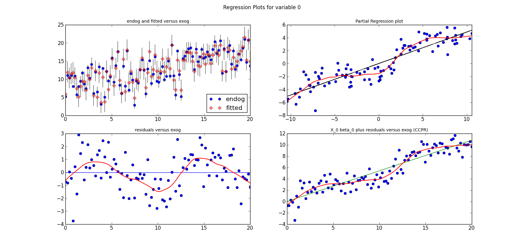
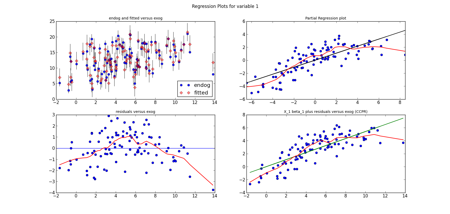
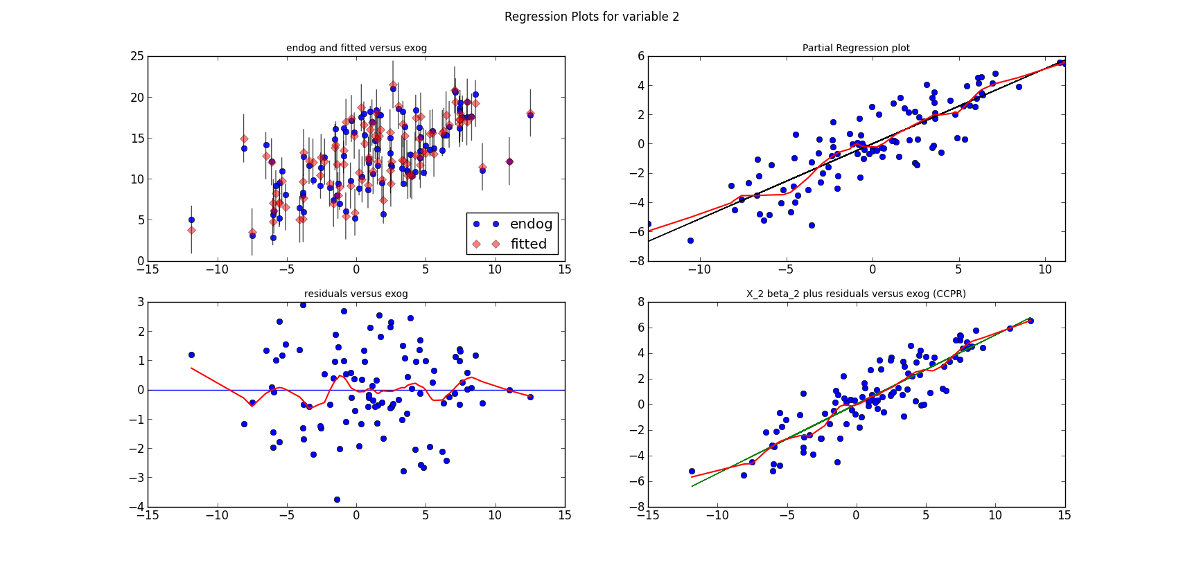
from regressionplots_new import plot_regress_exog

fig9 = plot_regress_exog(res, exog_idx=0)
add_lowess(fig9, ax_idx=1, lines_idx=0)
add_lowess(fig9, ax_idx=2, lines_idx=0)
add_lowess(fig9, ax_idx=3, lines_idx=0)

fig10 = plot_regress_exog(res, exog_idx=1)
add_lowess(fig10, ax_idx=1, lines_idx=0)
add_lowess(fig10, ax_idx=2, lines_idx=0)
add_lowess(fig10, ax_idx=3, lines_idx=0)

fig11 = plot_regress_exog(res, exog_idx=2)
add_lowess(fig11, ax_idx=1, lines_idx=0)
add_lowess(fig11, ax_idx=2, lines_idx=0)
add_lowess(fig11, ax_idx=3, lines_idx=0)

Plots in statsmodels: qqplot

Other news first, since I haven't managed to catch up with the blogs:

• statsmodels has four students in GSoC, the first four projects described in my previous post. Congratulations to Alexandre, Divyanshu, George and Justin
• statsmodels 0.4.0 has been release with new name without scikits in front, more on pypi

statsmodels has a graphics subdirectory, where we started to collect some of the common statistical plots. To make the documentation a bit more exciting, I am adding plots directly to the docstrings for the individual functions. Currently, we don't have many of them in the online documentation yet, two examples violin_plot and bean_plot.
A note on the documentation: Skipper improved the frontpage, which makes it easier to find the documentation for the latest released version and for the development version. Currently, the development version is better and is improving, and it is incompatible with the 0.4.0 release in only one part.

quantile-quantile plot: qqplot

The documentation for the function is here. The function signature is

qqplot(data, dist=stats.norm, distargs=(), a=0, loc=0, scale=1, fit=False, line=False, ax=None)

I am not copying the entire docstring, what I would like to present here are some examples and how to work with the plots.
The first example is from the docstring. I don't like the default, so I kept adding keyword arguments until the plot is more to my taste.

• The first plot uses no keywords and assumes normal distribution, and does not standardize the data.
• The second plot adds line='s', which according to the docstring

  's' - standardized line, the expected order statistics are scaled
        by the standard deviation of the given sample and have the mean
        added to them
  

  corresponds to the line after fitting location and scale for the normal distribution
• The third plot adds fit=True to get standardized sample quantiles and plots the 45 degree line. That's the plot I would prefer.
• The fourth plot is similar to the third plot, but with the t distribution instead of the normal distribution. I was surprised that the third and fourth plot look the same, until I checked and it turned out that the fitted t distribution has a huge degrees of freedom parameter and so is essentially identical to the normal distribution.

I will go over the code to produce this below.
I started the second example to see whether fitting the t distribution works correctly. Instead of using real data, I generate 1000 observations with a t distribution with df=4 and standard location(0) and scale (1).

• The first plot fits a normal distribution, keywords: line='45', fit=True
• The second plot fits the t distribution, keywords: dist=stats.t, line='45', fit=True
• The third plot is the same as the second plot, but I fit the t distribution myself, instead of having qqplot do it. keywords: dist=stats.t, distargs=(dof,), loc=loc, scale=scale, line='45'. I added the estimated parameters into a text insert in the plot. qqplot currently doesn't tell us what the fitted parameters are.

The Code

Here was my first attempt, following the docstring example

from scipy import stats
import statsmodels.api as sm

#estimate to get the residuals
data = sm.datasets.longley.load()
data.exog = sm.add_constant(data.exog)
mod_fit = sm.OLS(data.endog, data.exog).fit()
res = mod_fit.resid

fig = sm.graphics.qqplot(res, dist=stats.t, line='45', fit=True)
fig.show()

It works but the x-axis goes from -3 to 3, while there are only values from -2 to 2.

Detour to some background

A while ago we had a discussion on the mailing list what a plot in statsmodels should return. With the helpful comments of John Hunter, we finally agreed that plots should take an ax (matplotlib axis) argument if it's meaningful, and always return a figure instance fig. If ax is None, or the plot is a combination plot (several plots in one figure), then a figure is created and returned. If ax is given, then that is used to attach the plot elements. Ralf Gommers converted our plot functions to follow this pattern, besides that, he also wrote several of the plots that are currently in statsmodels.
So, to change the axis limits in the above graph, all I have to add is:

fig.axes[0].set_xlim(-2, 2)

The resulting plot is then the same as the third plot in the first graph above.

The first graph

Here is now the script for the first graph in several stages:
First I import some modules and calculate the residuals following the example

from scipy import stats
from matplotlib import pyplot as plt
import statsmodels.api as sm

#example from docstring
data = sm.datasets.longley.load()
data.exog = sm.add_constant(data.exog)
mod_fit = sm.OLS(data.endog, data.exog).fit()
res = mod_fit.resid

Then I hardcode a left position for text inserts, and create a matplotlib figure instance

left = -1.8
fig = plt.figure()

Next we can add the first subplot. The only keyword arguments for qqplot is ax to tell qqplot to attach the plot to my first subplot. Since I want to insert a text to describe the keywords, I needed to spend some time with the matplotlib documentation. As we have a reference to the axis instance, it is easy to change or add plot elements

ax = fig.add_subplot(2, 2, 1)
sm.graphics.qqplot(res, ax=ax)
top = ax.get_ylim()[1] * 0.75
txt = ax.text(left, top, 'no keywords', verticalalignment='top')
txt.set_bbox(dict(facecolor='k', alpha=0.1))

The other subplots follow the same pattern. I didn't try to generalize or avoid hardcoding

ax = fig.add_subplot(2, 2, 2)
sm.graphics.qqplot(res, line='s', ax=ax)
top = ax.get_ylim()[1] * 0.75
txt = ax.text(left, top, "line='s'", verticalalignment='top')
txt.set_bbox(dict(facecolor='k', alpha=0.1))

ax = fig.add_subplot(2, 2, 3)
sm.graphics.qqplot(res, line='45', fit=True, ax=ax)
ax.set_xlim(-2, 2)
top = ax.get_ylim()[1] * 0.75
txt = ax.text(left, top, "line='45', \nfit=True", verticalalignment='top')
txt.set_bbox(dict(facecolor='k', alpha=0.1))

ax = fig.add_subplot(2, 2, 4)
sm.graphics.qqplot(res, dist=stats.t, line='45', fit=True, ax=ax)
ax.set_xlim(-2, 2)
top = ax.get_ylim()[1] * 0.75
txt = ax.text(left, top, "dist=stats.t, \nline='45', \nfit=True",
              verticalalignment='top')
txt.set_bbox(dict(facecolor='k', alpha=0.1))

The final step is to adjust the layout, so that axis labels don't overlap with other subplots if the graph is not very large

fig.tight_layout()

The second graph

The second graph follows the same pattern with a few changes.
First we generate a random sample using scipy.stats which under the hood uses the random numbers from numpy. You can notice here that I am cheating. I ran the script several times to find "nice" seeds. Especially in smaller samples, qqplot might often not be very good in distinguishing normal and t distributions.

import numpy as np
seed = np.random.randint(1000000)
print 'seed', seed
seed = 461970  #nice seed for nobs=1000
#seed = 571478  #nice seed for nobs=100
#seed = 247819  #for nobs=100, estimated t is essentially normal
np.random.seed(seed)
rvs = stats.t.rvs(4, size=1000)

The first two subplot are very similar to what is in the first graph

fig2 = plt.figure()
ax = fig2.add_subplot(2, 2, 1)
fig2 = sm.graphics.qqplot(rvs, dist=stats.norm, line='45', fit=True, ax=ax)
top = ax.get_ylim()[1] * 0.75
xlim = ax.get_xlim()
frac = 0.1
left = xlim[0] * (1-frac) + xlim[1] * frac
txt = ax.text(left, top, "normal", verticalalignment='top')
txt.set_bbox(dict(facecolor='k', alpha=0.1))

ax = fig2.add_subplot(2, 2, 2)
fig2 = sm.graphics.qqplot(rvs, dist=stats.t, line='45', fit=True, ax=ax)
top = ax.get_ylim()[1] * 0.75
xlim = ax.get_xlim()
frac = 0.1
left = xlim[0] * (1-frac) + xlim[1] * frac
txt = ax.text(left, top, "t", verticalalignment='top')
txt.set_bbox(dict(facecolor='k', alpha=0.1))

For the third plot, I estimate the parameters of the t-distribution to see whether I get the same results as in the second plot (I do), and so I can insert the parameter estimates into the plot

params = stats.t.fit(rvs)
dof, loc, scale = params
ax = fig2.add_subplot(2, 2, 4)
fig2 = sm.graphics.qqplot(rvs, dist=stats.t, distargs=(dof,), loc=loc,
                 scale=scale, line='45', fit=False, ax=ax)
top = ax.get_ylim()[1] * 0.75
xlim = ax.get_xlim()
frac = 0.1
left = xlim[0] * (1-frac) + xlim[1] * frac
txt = ax.text(left, top, "t \ndof=%3.2F \nloc=%3.2F, \nscale=%3.2F" % tuple(params),
              verticalalignment='top')
txt.set_bbox(dict(facecolor='k', alpha=0.1))

That's it for the plots, now I need to add them to the statsmodels documentation.

PS: normality tests, details left for another day

qqplots give us a visual check whether a sample follows a specific distribution. The case that we are interested in most often, is a test for normality. Scipy.stats and statsmodels have several normality tests. The ones I have written recently are Anderson-Darling and Lillifors. Lillifors is a Kolmogorov-Smirnov test for normality when mean and variance are estimated. Calculating a statistical test provides a more reliable test than a "vague" visual inspection, but these tests do not point us to a specific alternative and provide less information about the direction in which a null hypothesis might be incorrect.
Using the residuals in the first example, neither test rejects the Null Hypothesis that the residuals come from a normal distribution

>>> normal_ad(res)
(0.43982328207860633, 0.25498161947268855)
>>> lillifors(res)
(0.17229856392873188, 0.2354638181341876)

On the other hand, in the second example with 1000 observations from the t distribution, the assumption that the data comes from a normal distribution is clearly rejected

>>> normal_ad(rvs)
(6.5408483355136013, 4.7694160497092537e-16)
>>> lillifors(rvs)
(0.05919821253474411, 8.5872265678140885e-09)

PPS:
I'm reluctant to publish the import path, because I had forgotten to add them to a proper place for 0.4.0, and the import location will not stay where it is. It took me a few minutes to find out that they are not on any recommended import path when I wrote these scripts

>>> from statsmodels.stats.adnorm import normal_ad
>>> from statsmodels.stats.lilliefors import lillifors

Statsmodels and Google Summer of Code 2012

I didn't have much time or motivation to work on my blog these last weeks, mainly because I was busy discussing Google Summer of Code and preparing a new release for statsmodels.

So here is just an update on our Google Summer of Code candidates and their projects. This year was a successful year in attracting student proposals. We have six proposals, five of them we discussed quite extensively on our mailing list before the application.

Of the five projects, the first two are must-haves for econometrics or statistical packages, one on System of Equations, the other on Nonlinear Least-Squares and Nonlinear Robust Models. The next two are nonparametric or semi-parametric methods, one more traditional kernel estimation, the other using Empirical Likelihood which is a relatively new approach that has become popular in recent research both in econometrics and in statistics. The fifth is on Dynamic Linear Models mainly using Kalman filter and a Bayesian approach, which would extend the depth of statsmodels in time series analysis.

All topics would be valuable extensions to statsmodels and significantly increase our coverage of statistics and econometrics. From the discussion on the mailing list I think that all candidates are qualified to bring the projects to a successful finish.

Estimating System of Equations

This is a standard econometrics topic, but I only recently found that graphical models and causal models discussed in other fields have a large overlap with this. In the case of a system of simultaneous equations, we have several variables that depend on each other. The simplest case in economics is a market equilibrium, where the demanded and supplied quantities depend on the price, and the price depends on the supply and demand. The estimation methods commonly used in this area are two-stage and three-stage least-squares and limited and full information maximum likelihood estimation. The first part of the project starts with the simpler case when we have several response variables, but they don't depend on each other simultaneously, although they can depend on past values of other response variables. I'm very glad that someone is picking this one up.

Extension of Linear to Non Linear Models

This project has two parts, the first is extending the linear least-squares model to the non-linear case, the second part is to implement non-linear models for robust estimation. Non-linear least squares is available in scipy for example with scipy.optimize.curve_fit. However, in the statsmodels version we want to provide all the usual results statistics and statistical tests. The second part will implement two robust estimators for non-linear model, that have been shown to be most successful in recent Monte Carlo studies comparing different robust estimators for non-linear equations. Robust estimation here refers to the case when there are possibly many outliers in the data. My guess is that these will become the most used models of all proposals.

Nonparametric Estimation

This project extends the kernel based method in statsmodels from the univariate to the multivariate case, will provide better bandwidth selection, and then implement nonparametric function estimation. Multivariate kernel density estimation should complement scipy.stats.gaussian_kde which only works well with distributions that are approximately normal shaped or have only a single peak. Another extension is to provide kernels and estimation methods for discrete variables. These methods have been on our wishlist for a while, but only the univariate case has been included in statsmodels so far.

Empirical Likelihood

This is a relatively new approach in statistics and econometrics that avoids the distributional assumptions in estimation and in statistical tests. Instead of relying on a known distribution in small samples, where we often assume normal distribution, or instead of relying on the asymptotic normal distribution in large samples, this approach estimates the distribution in a nonparametric way. This is similar, to some extend, to the difference between, for example, a t-test and a rank-based Mann–Whitney U or Wilcoxon test, which are available in scipy.stats. The advantages are that in smaller samples the estimates and tests are more accurate when the distribution is not known, and in many cases, for example in finance, most tests show that the assumption of normal distribution does not hold. For this project, I still have to catch up with some readings because I'm only familiar with a small part of this literature, mainly on empirical likelihood in relation to Generalized Method of Moments (GMM).

Dynamic Linear Models

This covers statespace models implemented by Kalman Filter for multivariate time series models, both from a likelihood and a Bayesian perspective. The project expands the coverage of statsmodels in linear time series analysis, the first area where we get a good coverage of models. Currently, we have univariate AR and ARIMA, vector autoregressive models VAR, and structural VAR. Part of this project would be to get a good cython based implementation of Kalman filters. Wes has started a libray, statlib, for this last year, however, it is still incomplete and needs to be integrated with statsmodels. Another advantage of this project is that it increases our infrastructure and models for macro-econometrics, estimation of macroeconomic models and dynamic stochastic general equilibrium DSGE models, which is currently still Matlab dominated, as far as I can tell.

Now we still have to see how many GSoC slots we will get, but we have the chance this year to get a large increase in the speed of development of statsmodels, and we can reduce the number of cases where someone needs to run to R, or Stata, or Matlab because there is no implementation for a statistical analysis available in Python.