Regression Plots - Part 1

I started to work on improving the documentation for the regressions plot in statsmodels. (However, I realized I have to improve them a bit.)

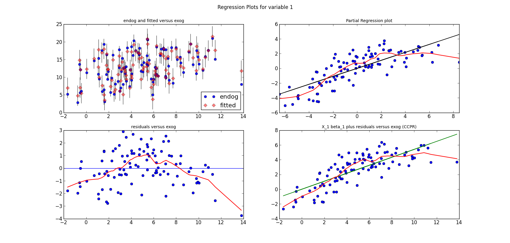
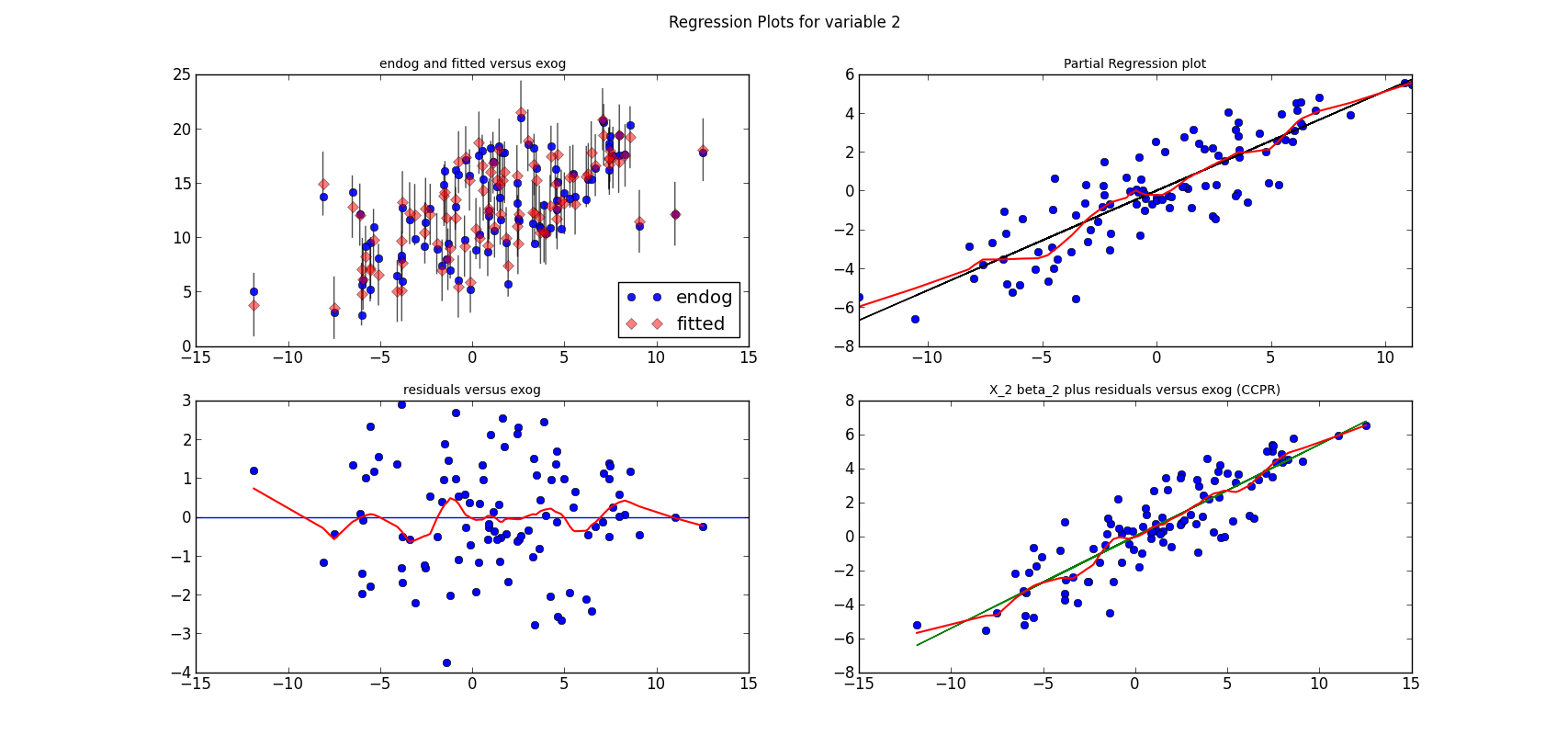
For now, just a question: Can you spot the mis-specification of the model?

I simulate a model, run a linear regression on three variables and a constant. Here is the estimation summary, which looks quite good, large R-squared, all variables significant, no obvious problems:

>>> print res.summary()
                                                        OLS Regression Results
==============================================================================
Dep. Variable:                      y   R-squared:                       0.901
Model:                            OLS   Adj. R-squared:                  0.898
Method:                 Least Squares   F-statistic:                     290.3
Date:                Thu, 10 May 2012   Prob (F-statistic):           5.31e-48
Time:                        13:15:22   Log-Likelihood:                -173.85
No. Observations:                 100   AIC:                             355.7
Df Residuals:                      96   BIC:                             366.1
Df Model:                           3
==============================================================================
                 coef    std err          t      P>|t|      [95.0% Conf. Int.]
------------------------------------------------------------------------------
x1             0.4872      0.024     20.076      0.000         0.439     0.535
x2             0.5408      0.045     12.067      0.000         0.452     0.630
x3             0.5136      0.030     16.943      0.000         0.453     0.574
const          4.6294      0.372     12.446      0.000         3.891     5.368
==============================================================================
Omnibus:                        0.945   Durbin-Watson:                   1.570
Prob(Omnibus):                  0.624   Jarque-Bera (JB):                1.031
Skew:                          -0.159   Prob(JB):                        0.597
Kurtosis:                       2.617   Cond. No.                         33.2
==============================================================================

The following three graphs are refactored versions of the regression plots. Each graph looks at the data and estimation results with respect to one of the three variables. (The graphs look better in original size.)
The short lines in the first subplot of each graph are the prediction confidence intervals for each observation.
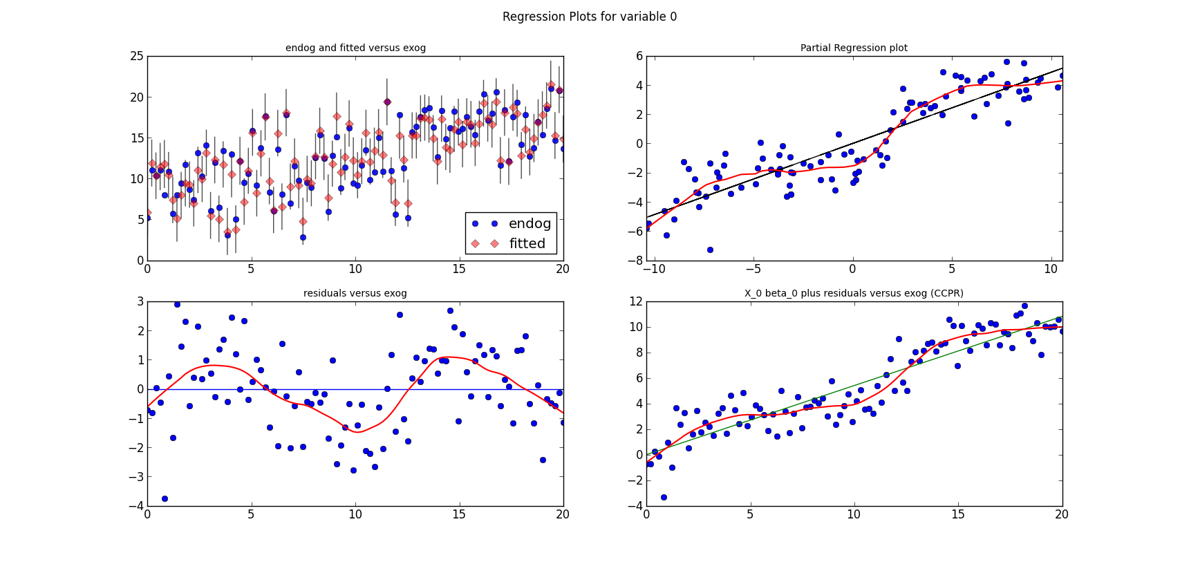
The code is short, if we have the (still unpublished) helper functions.
res is an OLS results instance

from regressionplots_new import plot_regress_exog

fig9 = plot_regress_exog(res, exog_idx=0)
add_lowess(fig9, ax_idx=1, lines_idx=0)
add_lowess(fig9, ax_idx=2, lines_idx=0)
add_lowess(fig9, ax_idx=3, lines_idx=0)

fig10 = plot_regress_exog(res, exog_idx=1)
add_lowess(fig10, ax_idx=1, lines_idx=0)
add_lowess(fig10, ax_idx=2, lines_idx=0)
add_lowess(fig10, ax_idx=3, lines_idx=0)

fig11 = plot_regress_exog(res, exog_idx=2)
add_lowess(fig11, ax_idx=1, lines_idx=0)
add_lowess(fig11, ax_idx=2, lines_idx=0)
add_lowess(fig11, ax_idx=3, lines_idx=0)

Plots in statsmodels: qqplot

Other news first, since I haven't managed to catch up with the blogs:

• statsmodels has four students in GSoC, the first four projects described in my previous post. Congratulations to Alexandre, Divyanshu, George and Justin
• statsmodels 0.4.0 has been release with new name without scikits in front, more on pypi

statsmodels has a graphics subdirectory, where we started to collect some of the common statistical plots. To make the documentation a bit more exciting, I am adding plots directly to the docstrings for the individual functions. Currently, we don't have many of them in the online documentation yet, two examples violin_plot and bean_plot.
A note on the documentation: Skipper improved the frontpage, which makes it easier to find the documentation for the latest released version and for the development version. Currently, the development version is better and is improving, and it is incompatible with the 0.4.0 release in only one part.

quantile-quantile plot: qqplot

The documentation for the function is here. The function signature is

qqplot(data, dist=stats.norm, distargs=(), a=0, loc=0, scale=1, fit=False, line=False, ax=None)

I am not copying the entire docstring, what I would like to present here are some examples and how to work with the plots.
The first example is from the docstring. I don't like the default, so I kept adding keyword arguments until the plot is more to my taste.

• The first plot uses no keywords and assumes normal distribution, and does not standardize the data.
• The second plot adds line='s', which according to the docstring

  's' - standardized line, the expected order statistics are scaled
        by the standard deviation of the given sample and have the mean
        added to them
  

  corresponds to the line after fitting location and scale for the normal distribution
• The third plot adds fit=True to get standardized sample quantiles and plots the 45 degree line. That's the plot I would prefer.
• The fourth plot is similar to the third plot, but with the t distribution instead of the normal distribution. I was surprised that the third and fourth plot look the same, until I checked and it turned out that the fitted t distribution has a huge degrees of freedom parameter and so is essentially identical to the normal distribution.

I will go over the code to produce this below.
I started the second example to see whether fitting the t distribution works correctly. Instead of using real data, I generate 1000 observations with a t distribution with df=4 and standard location(0) and scale (1).

• The first plot fits a normal distribution, keywords: line='45', fit=True
• The second plot fits the t distribution, keywords: dist=stats.t, line='45', fit=True
• The third plot is the same as the second plot, but I fit the t distribution myself, instead of having qqplot do it. keywords: dist=stats.t, distargs=(dof,), loc=loc, scale=scale, line='45'. I added the estimated parameters into a text insert in the plot. qqplot currently doesn't tell us what the fitted parameters are.

The Code

Here was my first attempt, following the docstring example

from scipy import stats
import statsmodels.api as sm

#estimate to get the residuals
data = sm.datasets.longley.load()
data.exog = sm.add_constant(data.exog)
mod_fit = sm.OLS(data.endog, data.exog).fit()
res = mod_fit.resid

fig = sm.graphics.qqplot(res, dist=stats.t, line='45', fit=True)
fig.show()

It works but the x-axis goes from -3 to 3, while there are only values from -2 to 2.

Detour to some background

A while ago we had a discussion on the mailing list what a plot in statsmodels should return. With the helpful comments of John Hunter, we finally agreed that plots should take an ax (matplotlib axis) argument if it's meaningful, and always return a figure instance fig. If ax is None, or the plot is a combination plot (several plots in one figure), then a figure is created and returned. If ax is given, then that is used to attach the plot elements. Ralf Gommers converted our plot functions to follow this pattern, besides that, he also wrote several of the plots that are currently in statsmodels.
So, to change the axis limits in the above graph, all I have to add is:

fig.axes[0].set_xlim(-2, 2)

The resulting plot is then the same as the third plot in the first graph above.

The first graph

Here is now the script for the first graph in several stages:
First I import some modules and calculate the residuals following the example

from scipy import stats
from matplotlib import pyplot as plt
import statsmodels.api as sm

#example from docstring
data = sm.datasets.longley.load()
data.exog = sm.add_constant(data.exog)
mod_fit = sm.OLS(data.endog, data.exog).fit()
res = mod_fit.resid

Then I hardcode a left position for text inserts, and create a matplotlib figure instance

left = -1.8
fig = plt.figure()

Next we can add the first subplot. The only keyword arguments for qqplot is ax to tell qqplot to attach the plot to my first subplot. Since I want to insert a text to describe the keywords, I needed to spend some time with the matplotlib documentation. As we have a reference to the axis instance, it is easy to change or add plot elements

ax = fig.add_subplot(2, 2, 1)
sm.graphics.qqplot(res, ax=ax)
top = ax.get_ylim()[1] * 0.75
txt = ax.text(left, top, 'no keywords', verticalalignment='top')
txt.set_bbox(dict(facecolor='k', alpha=0.1))

The other subplots follow the same pattern. I didn't try to generalize or avoid hardcoding

ax = fig.add_subplot(2, 2, 2)
sm.graphics.qqplot(res, line='s', ax=ax)
top = ax.get_ylim()[1] * 0.75
txt = ax.text(left, top, "line='s'", verticalalignment='top')
txt.set_bbox(dict(facecolor='k', alpha=0.1))

ax = fig.add_subplot(2, 2, 3)
sm.graphics.qqplot(res, line='45', fit=True, ax=ax)
ax.set_xlim(-2, 2)
top = ax.get_ylim()[1] * 0.75
txt = ax.text(left, top, "line='45', \nfit=True", verticalalignment='top')
txt.set_bbox(dict(facecolor='k', alpha=0.1))

ax = fig.add_subplot(2, 2, 4)
sm.graphics.qqplot(res, dist=stats.t, line='45', fit=True, ax=ax)
ax.set_xlim(-2, 2)
top = ax.get_ylim()[1] * 0.75
txt = ax.text(left, top, "dist=stats.t, \nline='45', \nfit=True",
              verticalalignment='top')
txt.set_bbox(dict(facecolor='k', alpha=0.1))

The final step is to adjust the layout, so that axis labels don't overlap with other subplots if the graph is not very large

fig.tight_layout()

The second graph

The second graph follows the same pattern with a few changes.
First we generate a random sample using scipy.stats which under the hood uses the random numbers from numpy. You can notice here that I am cheating. I ran the script several times to find "nice" seeds. Especially in smaller samples, qqplot might often not be very good in distinguishing normal and t distributions.

import numpy as np
seed = np.random.randint(1000000)
print 'seed', seed
seed = 461970  #nice seed for nobs=1000
#seed = 571478  #nice seed for nobs=100
#seed = 247819  #for nobs=100, estimated t is essentially normal
np.random.seed(seed)
rvs = stats.t.rvs(4, size=1000)

The first two subplot are very similar to what is in the first graph

fig2 = plt.figure()
ax = fig2.add_subplot(2, 2, 1)
fig2 = sm.graphics.qqplot(rvs, dist=stats.norm, line='45', fit=True, ax=ax)
top = ax.get_ylim()[1] * 0.75
xlim = ax.get_xlim()
frac = 0.1
left = xlim[0] * (1-frac) + xlim[1] * frac
txt = ax.text(left, top, "normal", verticalalignment='top')
txt.set_bbox(dict(facecolor='k', alpha=0.1))

ax = fig2.add_subplot(2, 2, 2)
fig2 = sm.graphics.qqplot(rvs, dist=stats.t, line='45', fit=True, ax=ax)
top = ax.get_ylim()[1] * 0.75
xlim = ax.get_xlim()
frac = 0.1
left = xlim[0] * (1-frac) + xlim[1] * frac
txt = ax.text(left, top, "t", verticalalignment='top')
txt.set_bbox(dict(facecolor='k', alpha=0.1))

For the third plot, I estimate the parameters of the t-distribution to see whether I get the same results as in the second plot (I do), and so I can insert the parameter estimates into the plot

params = stats.t.fit(rvs)
dof, loc, scale = params
ax = fig2.add_subplot(2, 2, 4)
fig2 = sm.graphics.qqplot(rvs, dist=stats.t, distargs=(dof,), loc=loc,
                 scale=scale, line='45', fit=False, ax=ax)
top = ax.get_ylim()[1] * 0.75
xlim = ax.get_xlim()
frac = 0.1
left = xlim[0] * (1-frac) + xlim[1] * frac
txt = ax.text(left, top, "t \ndof=%3.2F \nloc=%3.2F, \nscale=%3.2F" % tuple(params),
              verticalalignment='top')
txt.set_bbox(dict(facecolor='k', alpha=0.1))

That's it for the plots, now I need to add them to the statsmodels documentation.

PS: normality tests, details left for another day

qqplots give us a visual check whether a sample follows a specific distribution. The case that we are interested in most often, is a test for normality. Scipy.stats and statsmodels have several normality tests. The ones I have written recently are Anderson-Darling and Lillifors. Lillifors is a Kolmogorov-Smirnov test for normality when mean and variance are estimated. Calculating a statistical test provides a more reliable test than a "vague" visual inspection, but these tests do not point us to a specific alternative and provide less information about the direction in which a null hypothesis might be incorrect.
Using the residuals in the first example, neither test rejects the Null Hypothesis that the residuals come from a normal distribution

>>> normal_ad(res)
(0.43982328207860633, 0.25498161947268855)
>>> lillifors(res)
(0.17229856392873188, 0.2354638181341876)

On the other hand, in the second example with 1000 observations from the t distribution, the assumption that the data comes from a normal distribution is clearly rejected

>>> normal_ad(rvs)
(6.5408483355136013, 4.7694160497092537e-16)
>>> lillifors(rvs)
(0.05919821253474411, 8.5872265678140885e-09)

PPS:
I'm reluctant to publish the import path, because I had forgotten to add them to a proper place for 0.4.0, and the import location will not stay where it is. It took me a few minutes to find out that they are not on any recommended import path when I wrote these scripts

>>> from statsmodels.stats.adnorm import normal_ad
>>> from statsmodels.stats.lilliefors import lillifors

Using rst2blogger and Breush-Godfrey test

This is mainly a test to see if rst2blogger works. The description sounded like just what I needed to make going from rst file to blogger less work. Some setup inconveniences: Why do python programs need to install distribute and destroy my setuptools? Lxml didn't have windows binaries, and easy_install fails because the source doesn't build. In contrast to sphinx, the plain docutils do not highlight python code, at least not right away. If there is an exception in rendering the html, then the message is completely uninformative: except Exception

(Reminds me of the sound I'm hearing when the kids are just guessing in a numbers game: "Try again", "Try again", ...)

try a rst list: some categories of tests that I have been working on recently.

• diagnostic tests
  • autocorrelation
  • heteroscedasticity
  • multicollinearity
  • functional form
  • normality
  • outliers
  • influence
• tests for coefficients/parameters
  • t test for linear restrictions
  • F test for linear restrictions
  • Wald test for linear restrictions missing
  • Likelihood Ratio test to compare nested models
  • Wald/F test test to compare nested models
  • comparing non-nested models: J, Cox

Writing Breush-Godfrey autocorrelation test in 5 minutes

The background story: I have written several diagnostics tests a while ago, maybe one and a half years ago. Many of the diagnostic test have a similar structure and it's easy to just copy the pattern. For one test, acorr_lm, I took the code and basic idea of the augmented dickey fuller test for unit roots, and wanted to make a Lagrange Multiplier test for autocorrelation out of it. Some time later, I added some comments that this could be used as Engle's ARCH test but that there is a difference to Breush-Godfrey's serial correlation test.

While I was writing tests comparing my diagnostic tests with R, I saw that Breush-Godfrey was still missing. Since this time I had unit tests, it was very quick work, copy and paste, and checking Wikipedia .

The test passed after a few changes, and I barely had to think.

Build the matrix of lagged residuals, column_stack them with the original regressors, get the matrix for the linear restrictions that the joint effect of the lagged residuals is zero. Most of the work is done by existing functions.

I haven't changed the docstring yet, and there is still cleanup work to do.

def acorr_breush_godfrey(results, nlags=None, store=False):
    '''Lagrange Multiplier tests for autocorrelation

    not checked yet, copied from unitrood_adf with adjustments
    check array shapes because of the addition of the constant.
    written/copied without reference
    This is not Breush-Godfrey. BG adds lags of residual to exog in the
    design matrix for the auxiliary regression with residuals as endog,
    see Greene 12.7.1.

    Notes
    -----
    If x is calculated as y^2 for a time series y, then this test corresponds
    to the Engel test for autoregressive conditional heteroscedasticity (ARCH).
    TODO: get details and verify

    '''

    x = np.concatenate((np.zeros(nlags), results.resid))
    exog_old = results.model.exog
    x = np.asarray(x)
    nobs = x.shape[0]
    if nlags is None:
        #for adf from Greene referencing Schwert 1989
        nlags = 12. * np.power(nobs/100., 1/4.)#nobs//4  #TODO: check default, or do AIC/BIC

    xdall = lagmat(x[:,None], nlags, trim='both')
    nobs = xdall.shape[0]
    xdall = np.c_[np.ones((nobs,1)), xdall]
    xshort = x[-nobs:]
    exog = np.column_stack((exog_old, xdall))
    k_vars = exog.shape[1]

    if store: resstore = ResultsStore()

    resols = sm.OLS(xshort, exog).fit()
    ft = resols.f_test(np.eye(nlags, k_vars, k_vars - nlags))
    fval = ft.fvalue
    fpval = ft.pvalue
    fval = np.squeeze(fval)[()]   #TODO: fix this in ContrastResults
    fpval = np.squeeze(fpval)[()]
    lm = nobs * resols.rsquared
    lmpval = stats.chi2.sf(lm, nlags)
    # Note: degrees of freedom for LM test is nvars minus constant = usedlags
    #return fval, fpval, lm, lmpval

    if store:
        resstore.resols = resols
        resstore.usedlag = nlags
        return fval, fpval, lm, lmpval, resstore
    else:
        return fval, fpval, lm, lmpval

Just a brief explanation to the main tools:

lagmat just creates a matrix of lagged values without having to worry about how to shift and cut the arrays.

>>> from scikits.statsmodels.tsa.tsatools import lagmat
>>> lagmat(np.arange(8), 3, trim='both')
array([[ 2.,  1.,  0.],
       [ 3.,  2.,  1.],
       [ 4.,  3.,  2.],
       [ 5.,  4.,  3.],
       [ 6.,  5.,  4.]])

numpy.eye is very flexible and allows shifting of the diagonal

>>> np.eye(3, 5, 5-3)
array([[ 0.,  0.,  1.,  0.,  0.],
       [ 0.,  0.,  0.,  1.,  0.],
       [ 0.,  0.,  0.,  0.,  1.]])

The rest are mainly calls to OLS and f_test. One part I needed to change was that R takes the initial errors to be zero instead of truncating the regression, so I also had to concatenate some zeros in front of the regression residuals array.

Starting a list of diagnostic and specification tests

I started already several times an inventory of statistical tests in python, scipy.stats and statsmodels, compared to R.

Here is another try.

It is mainly the comparison with the R package lmtest. I just spend most of two days, writing tests against R, and before that some days of writing tests against Gretl, and before that outlier measures against SAS, as described in the previous posts.

I don't know yet how easy it will be to maintain a list like this, the current version is mainly based on parsing the lmtest index page. lmtest is not very complete, and there are tests covered in other packages and additional tests covered in Gretl.

For now I just keep it in a boring python module, with a string that's easy to manipulate and convert.

#cols: category, name, statsmodels, r_lmtest, gretl

s4 = '''\

acorr | Breusch-Godfrey Test | acorr_breush_godfrey | bgtest

acorr | Durbin-Watson Test | location_no_pvalues | dwtest

het | Breusch-Pagan Test | het_breush_pagan | bptest

het | Goldfeld-Quandt Test | het_goldfeld_quandt | gqtest

het | Harrison-McCabe test | missing | hmctest

het | White test | het_white | - |

causality | Test for Granger Causality | grangercausalitytest | grangertest

linear | Harvey-Collier Test | missing | harvtest

linear | PE Test for Linear vs. Log-Linear Specifications | missing | petest

linear | Rainbow Test | missing | raintest

func form | RESET Test | with outliers | resettest

compare nonnested | Cox Test | compare_cox | coxtest

compare nonnested | J Test | compare_j | jtest

compare nonnested | Encompassing Test | missing | encomptest

compare nested | Likelihood Ratio Test nested | compare_lr | lrtest

compare nested | Wald Test nested | compare_ftest | waldtest

coef | Testing Estimated Coefficients | t_test | coeftest

coef | Testing Estimated Coefficients | missing | coeftest.breakpointsfull

'''

add another separator

print '\n'.join(line + '|' for line in s4.split('\n'))

convert to list of list 

def str2list(ss, sep='|', keep_empty=4):

Unfortunately copying into blogger doesn't preserve intend, so skip this. And convert separator to tabs, so that google spreadsheet separates the cells:

print '\n'.join(line + '|' for line in s4.split('\n'))

Tomorrow, I will start looking for the diagnostic tests that are not yet on the list. R stats has some, for example (fm is my test case linear model result)

> names(ls.diag(fm))
 [1] "std.dev"      "hat"          "std.res"      "stud.res"     "cooks"        "dfits"      
 [7] "correlation"  "std.err"      "cov.scaled"   "cov.unscaled"

I figured out that json works pretty well transferring data from some R animals to python.

In other news:
The basic R doesn't save automatically the sessionlog or history. I was playing with Rcommander last night to see what default diagnostics they are proposing, and it crashed R after a while. Unfortunately, I hadn't saved my sessionlog and script file, so a day or two of work died with it. I didn't think about safeguarding against crashes anymore, Windows never crashes, not even the kids manage to turn it off anymore, spyder and firefox always recover after a crash with an existing history or session log. R never crashed before.

Anscombe and Diagnostic Statistics

Now that I got these outlier and influence measures (see last post), we can look at the Anscombe example, Anscombe Quartet

I took the example from matplotlib here. With a few changes, mainly adding the observation number. I get this graph

The first example is what we would usually expect and shouldn't have any problems for estimating the regression line. The second example is nonlinear, but we are fitting only a linear model. The third example has an outlier in y, which pulls the regression line towards it. The last example has an outlier in x.

Interpreting the last case is a bit tricky. The slope of the regression line is dominated by observation 7, if we think it is a reliable (correctly measured) observation, then it is very useful since it contains a lot of information. If we doubt the reliability of that measurement, then we are left without any information about the slope and the effect of the explanatory variable.
(I don't remember where I read this, someone argued that we shouldn't through out x outliers.)

Now we can run a loop over the four problems and check the influence diagnostic table, and also Ramsey's RESET test for linearity.

example 1: ok
-------------


Parameter estimates (constant, slope): [ 3.00009091  0.50009091]
=============================================================================================================
       obs      endog     fitted     Cook's   student.   hat diag    dffits   ext.stud.     dffits     dfbeta
                           value          d   residual              internal   residual                 slope
-------------------------------------------------------------------------------------------------------------
         0      8.040      8.001      0.000      0.033      0.100      0.011      0.031      0.010      0.003
         1      6.950      7.001      0.000     -0.043      0.100     -0.014     -0.041     -0.014      0.004
         2      7.580      9.501      0.489     -1.778      0.236     -0.989     -2.081     -1.158     -0.908
         3      8.810      7.501      0.062      1.110      0.091      0.351      1.127      0.356      0.000
         4      8.330      8.501      0.002     -0.148      0.127     -0.057     -0.140     -0.053     -0.029
         5      9.960     10.001      0.000     -0.041      0.318     -0.028     -0.038     -0.026     -0.022
         6      7.240      6.001      0.127      1.102      0.173      0.503      1.117      0.510     -0.351
         7      4.260      5.000      0.123     -0.725      0.318     -0.495     -0.705     -0.481      0.407
         8     10.840      9.001      0.279      1.635      0.173      0.747      1.838      0.840      0.578
         9      4.820      6.501      0.154     -1.455      0.127     -0.556     -1.569     -0.599      0.320
        10      5.680      5.500      0.004      0.166      0.236      0.092      0.157      0.087     -0.068
=============================================================================================================
RESET
F test: F=array([[ 0.44964358]]), p=[[ 0.77063577]], df_denom=5, df_num=4

Everything looks mostly ok, the RESET test doesn't reject the linear specification. Observation 2 might be an outlier, the studentized residual is at around 2, which is about the threshold for the t-distribution.

example 2: nonlinear
--------------------


Parameter estimates (constant, slope): [ 3.00090909  0.5       ]
=============================================================================================================
       obs      endog     fitted     Cook's   student.   hat diag    dffits   ext.stud.     dffits     dfbeta
                           value          d   residual              internal   residual                 slope
-------------------------------------------------------------------------------------------------------------
         0      9.140      8.001      0.052      0.971      0.100      0.324      0.967      0.322      0.097
         1      8.140      7.001      0.052      0.971      0.100      0.324      0.967      0.322     -0.097
         2      8.740      9.501      0.077     -0.704      0.236     -0.392     -0.683     -0.380     -0.298
         3      8.770      7.501      0.058      1.076      0.091      0.340      1.087      0.344      0.000
         4      9.260      8.501      0.032      0.657      0.127      0.251      0.635      0.242      0.130
         5      8.100     10.001      0.808     -1.861      0.318     -1.271     -2.236     -1.528     -1.291
         6      6.130      6.001      0.001      0.115      0.173      0.052      0.108      0.050     -0.034
         7      3.100      5.001      0.808     -1.861      0.318     -1.271     -2.236     -1.528      1.291
         8      9.130      9.001      0.001      0.115      0.173      0.052      0.108      0.050      0.034
         9      7.260      6.501      0.032      0.657      0.127      0.251      0.635      0.242     -0.130
        10      4.740      5.501      0.077     -0.704      0.236     -0.392     -0.683     -0.380      0.298
=============================================================================================================
RESET
F test: F=array([[ 820836.08290181]]), p=[[ 0.]], df_denom=5, df_num=4

Observation 2 and 7 look like outliers. However, the RESET test strongly rejects the hypothesis that the linear specification is correct. So we better look for another model, for example including polynomial terms for the explanatory variable.


example 3: outlier at 2
----------------------


Parameter estimates (constant, slope): [ 3.00245455  0.49972727]
=============================================================================================================
       obs      endog     fitted     Cook's   student.   hat diag    dffits   ext.stud.     dffits     dfbeta
                           value          d   residual              internal   residual                 slope
-------------------------------------------------------------------------------------------------------------
         0      7.460      8.000      0.012     -0.460      0.100     -0.153     -0.439     -0.146     -0.044
         1      6.770      7.000      0.002     -0.196      0.100     -0.065     -0.186     -0.062      0.019
         2     12.740      9.499      1.393      3.000      0.236      1.669   1203.540    669.587    525.268
         3      7.110      7.500      0.005     -0.331      0.091     -0.105     -0.314     -0.099      0.000
         4      7.810      8.499      0.026     -0.597      0.127     -0.228     -0.574     -0.219     -0.117
         5      8.840      9.999      0.301     -1.135      0.318     -0.775     -1.156     -0.790     -0.667
         6      6.080      6.001      0.001      0.070      0.173      0.032      0.066      0.030     -0.021
         7      5.390      5.001      0.034      0.381      0.318      0.260      0.362      0.247     -0.209
         8      8.150      8.999      0.059     -0.755      0.173     -0.345     -0.736     -0.336     -0.231
         9      6.420      6.500      0.000     -0.070      0.127     -0.027     -0.066     -0.025      0.013
        10      5.730      5.501      0.007      0.212      0.236      0.118      0.200      0.111     -0.087
=============================================================================================================
RESET
F test: F=array([[ 1.42791012]]), p=[[ 0.34730273]], df_denom=5, df_num=4

The results from the table are pretty clear, observation 2 has to be an outlier, all residual measures are huge. The RESET test doesn't indicate any problem with the linear specification.


example 4: exog_outlier at 7
----------------------------


Parameter estimates (constant, slope): [ 3.00172727  0.49990909]
=============================================================================================================
       obs      endog     fitted     Cook's   student.   hat diag    dffits   ext.stud.     dffits     dfbeta
                           value          d   residual              internal   residual                 slope
-------------------------------------------------------------------------------------------------------------
         0      6.580      7.001      0.007     -0.359      0.100     -0.120     -0.341     -0.114      0.034
         1      5.760      7.001      0.062     -1.059      0.100     -0.353     -1.067     -0.356      0.107
         2      7.710      7.001      0.020      0.605      0.100      0.202      0.582      0.194     -0.059
         3      8.840      7.001      0.137      1.569      0.100      0.523      1.735      0.578     -0.174
         4      8.470      7.001      0.087      1.253      0.100      0.418      1.300      0.433     -0.131
         5      7.040      7.001      0.000      0.033      0.100      0.011      0.031      0.011     -0.003
         6      5.250      7.001      0.124     -1.494      0.100     -0.498     -1.624     -0.541      0.163
         7     12.500     12.500     -1.#IO     -1.#IO      1.000     -1.#IO     -1.#IO     -1.#IO     -3.070
         8      5.560      7.001      0.084     -1.229      0.100     -0.410     -1.271     -0.423      0.128
         9      7.910      7.001      0.033      0.775      0.100      0.259      0.757      0.252     -0.076
        10      6.890      7.001      0.001     -0.095      0.100     -0.032     -0.089     -0.030      0.009
=============================================================================================================
RESET
F test: F=array([[ 126.84716907]]), p=[[ 0.00000007]], df_denom=9, df_num=4


What's going on with observation 7? The "-1.#IO" stands for numpy.NaN. All the measures that rely on leaving out observation 7 are indeterminate, since without observation 7 we cannot identify a slope.
The diagonal value of the hat matrix and the dfbeta for the slope indicate that this observation is very influential.
 

example 4a: exog_outlier at 7 (v2)
----------------------------------


Parameter estimates (constant, slope): [ 3.00172741  0.49990908]
=============================================================================================================
       obs      endog     fitted     Cook's   student.   hat diag    dffits   ext.stud.     dffits     dfbeta
                           value          d   residual              internal   residual                 slope
-------------------------------------------------------------------------------------------------------------
         0      7.006      7.006      0.000      0.000      0.091      0.000      0.000      0.000     -0.000
         1      6.580      7.001      0.007     -0.377      0.091     -0.119     -0.360     -0.114      0.033
         2      5.760      7.001      0.062     -1.110      0.091     -0.351     -1.125     -0.356      0.103
         3      7.710      7.001      0.020      0.634      0.091      0.201      0.614      0.194     -0.056
         4      8.840      7.001      0.135      1.645      0.091      0.520      1.828      0.578     -0.167
         5      8.470      7.001      0.086      1.314      0.091      0.416      1.371      0.434     -0.125
         6      7.040      7.001      0.000      0.035      0.091      0.011      0.033      0.011     -0.003
         7      5.250      7.001      0.123     -1.567      0.091     -0.495     -1.711     -0.541      0.156
         8     12.500     12.500      0.000     -0.000      1.000     -0.001     -0.000     -0.001     -0.001
         9      5.560      7.001      0.083     -1.289      0.091     -0.408     -1.339     -0.424      0.122
        10      7.910      7.001      0.033      0.813      0.091      0.257      0.798      0.253     -0.073
        11      6.890      7.001      0.001     -0.099      0.091     -0.031     -0.094     -0.030      0.009
=============================================================================================================
RESET
F test: F=array([[ 113.86707171]]), p=[[ 0.00000011]], df_denom=9, df_num=4

Since I didn't like the NaN results in the previous example, I made one change. I added an additional observation that has an x value slightly larger the the large group, 8.01 insted of 8.00, the y value was chosen so it lies on the predicted line. The new observation is the first observation, the x outlier is now at index 8.

What happened to our influence measures? Both observations 0 and 8 have zero influence, since we only need one of them to identify the slope. Leave one observation out doesn't help if we have two "similar" (in terms of parameter estimation) outliers.

Since this was interesting, let's try another variation. This time I change the value of the new observation to lie below the regression line (6.999 instead of 7.006). One more table and we are done.

example 4b: exog_outlier at 7 (v3)
----------------------------------


Parameter estimates (constant, slope): [ 3.00063327  0.49996637]
=============================================================================================================
       obs      endog     fitted     Cook's   student.   hat diag    dffits   ext.stud.     dffits     dfbeta
                           value          d   residual              internal   residual                 slope
-------------------------------------------------------------------------------------------------------------
         0      6.999      7.005      0.000     -0.006      0.091     -0.002     -0.005     -0.002      0.001
         1      6.580      7.000      0.007     -0.376      0.091     -0.119     -0.359     -0.114      0.033
         2      5.760      7.000      0.062     -1.110      0.091     -0.351     -1.124     -0.356      0.103
         3      7.710      7.000      0.020      0.635      0.091      0.201      0.615      0.194     -0.056
         4      8.840      7.000      0.136      1.646      0.091      0.520      1.829      0.578     -0.167
         5      8.470      7.000      0.086      1.315      0.091      0.416      1.372      0.434     -0.125
         6      7.040      7.000      0.000      0.035      0.091      0.011      0.034      0.011     -0.003
         7      5.250      7.000      0.123     -1.566      0.091     -0.495     -1.710     -0.541      0.156
         8     12.500     12.500     21.566      0.006      1.000      6.567      0.005      6.231      5.965
         9      5.560      7.000      0.083     -1.289      0.091     -0.407     -1.339     -0.423      0.122
        10      7.910      7.000      0.033      0.814      0.091      0.257      0.799      0.253     -0.073
        11      6.890      7.000      0.001     -0.099      0.091     -0.031     -0.094     -0.030      0.009
=============================================================================================================
RESET
F test: F=array([[ 113.85091319]]), p=[[ 0.00000011]], df_denom=9, df_num=4

Now we see that the outlier measures like the studentized residuals are very small for observation 8, however the influence measures, diagonal value of hat matrix, Cook's distance, dffits and dfbeta, are all large and clearly signal that this is a very influential observation.

Extra comment:

The RESET test in the versions of example four has different degrees of freedom than the first three examples, even though it uses the same code. After looking at this surprising result a bit, it turns out that because of the structure of the explanatory variable (only 2 or 3 distinct x values) the auxilliary regression for the RESET test has reduced rank.

A bit of history:
I didn't know about the Anscombe example until this thread http://mail.scipy.org/pipermail/scipy-user/2011-February/028462.html
It took me a year to get back to this.

Influence and Outlier measures in regression

Suppose we run a simple regression, and want to know whether there are possible outliers, or observations that have a large influence on the estimated parameters. In the past, I added several specification test to statsmodels. These are tests that check whether your model assumptions are "correct" or whether there are violations.
(This is sloppy phrasing, they are statistical tests after all.)

What is missing so far in statsmodels are the usual outlier and influence measures. (Although there are robust linear models.)

I found a nice example for influence and outlier measures using SAS in http://www.bios.unc.edu/~truong/b545/reg/simple/wa.html

Trying to do something similar as an extension to statsmodels, I ended up with the table below. This is supposed to correspond to the bottom tables on the above linked page.
All numbers look the same, but I'm still missing `Cov Ratio` and haven't looked for the prediction intervals yet. I also have dfbetas, but ran out of time to add them nicely to the table. Some of the measures have associated pvalues or recommended thresholds that can be used to interpret the results and find which observations might "mess up" the estimation.

Additionally, I also coded Variance Inflation Factor (VIF), a measure of multicollinearity for the explanatory variables, and the Ramsey RESET Test which is unrelated to the rest here and is a test for linear specification. I think I got now all from this page http://en.wikipedia.org/wiki/Category:Regression_diagnostics.

The code is roughly, after imports and estimating the model by OLS

infl = Influence(res_ols)

print infl.summary()

obs	endog	fitted	Cook's d	studentized	hat diag	dffits	ext.stud.	dffits
		value		residuals		internal	residuals
0.0	64.0	59.7143	0.0317	0.7513	0.1008	0.2516	0.7338	0.2457
1.0	71.0	67.0	0.0334	0.7079	0.1176	0.2585	0.6891	0.2516
2.0	53.0	52.4286	0.0025	0.1124	0.2857	0.0711	0.1067	0.0675
3.0	67.0	70.6429	0.058	-0.6778	0.2017	-0.3407	-0.6583	-0.3309
4.0	55.0	59.7143	0.0383	-0.8265	0.1008	-0.2768	-0.8123	-0.272
5.0	58.0	56.0714	0.0125	0.3515	0.1681	0.158	0.3355	0.1508
6.0	77.0	67.0	0.2088	1.7697	0.1176	0.6462	2.0259	0.7398
7.0	57.0	63.3571	0.0559	-1.1042	0.084	-0.3345	-1.1179	-0.3386
8.0	56.0	67.0	0.2526	-1.9467	0.1176	-0.7108	-2.3435	-0.8557
9.0	51.0	52.4286	0.0158	-0.281	0.2857	-0.1777	-0.2676	-0.1693
10.0	76.0	74.2857	0.031	0.3498	0.3361	0.2489	0.3339	0.2376
11.0	68.0	63.3571	0.0298	0.8064	0.084	0.2443	0.7912	0.2397

The html for this table was created with scikits.statsmodels.iolib.table.SimpleTable, but I never tried to fine tune the html options for a nice result. The text table that is getting printed in the python shell is

>>> print infl.summary_obs()
===================================================================================================
       obs      endog     fitted   Cook's d studentized   hat diag    dffits   ext.stud.     dffits
                           value              residuals              internal  residuals          
---------------------------------------------------------------------------------------------------
         0    64.0000    59.7143     0.0317      0.7513     0.1008     0.2516     0.7338     0.2457
         1    71.0000    67.0000     0.0334      0.7079     0.1176     0.2585     0.6891     0.2516
         2    53.0000    52.4286     0.0025      0.1124     0.2857     0.0711     0.1067     0.0675
         3    67.0000    70.6429     0.0580     -0.6778     0.2017    -0.3407    -0.6583    -0.3309
         4    55.0000    59.7143     0.0383     -0.8265     0.1008    -0.2768    -0.8123    -0.2720
         5    58.0000    56.0714     0.0125      0.3515     0.1681     0.1580     0.3355     0.1508
         6    77.0000    67.0000     0.2088      1.7697     0.1176     0.6462     2.0259     0.7398
         7    57.0000    63.3571     0.0559     -1.1042     0.0840    -0.3345    -1.1179    -0.3386
         8    56.0000    67.0000     0.2526     -1.9467     0.1176    -0.7108    -2.3435    -0.8557
         9    51.0000    52.4286     0.0158     -0.2810     0.2857    -0.1777    -0.2676    -0.1693
        10    76.0000    74.2857     0.0310      0.3498     0.3361     0.2489     0.3339     0.2376
        11    68.0000    63.3571     0.0298      0.8064     0.0840     0.2443     0.7912     0.2397
===================================================================================================


Observations 6 and 8 look like outliers from these measures.
 

This was the fun part, and I managed to get it done in a few (or more) hours this weekend. The rest sounds more like work.

Some comments on the implementation.

The first measures can be calculated efficiently from only the original regression, the second part of this list of measures requires a loop that estimates the model dropping each observation one at a time (Leave One Observation Out). The latter can get expensive if the number of observations is large.

Initially I wanted to cache all Leave One Observation Out result instances, but this might get expensive in terms of memory, since at least some copies of the data will be made and stored together with the result instances. Instead, I finally decided to loop once but store all the attributes that will be required for the various measures. (Right now, I actually needed only the estimate of the error variance and the parameter estimates).

If the number of observations is large, then calculating the Leave One Observation Out results for dropping every observation will be a waste, because many observations will not be likely candidates for the "full treatment". The, not yet implemented, idea is to calculate the cheap measures first, and use them to select those observations that are likely candidates for the more precise LOOO loop.

Also still missing: plots.
I did some cleanup for the regression plots, but the outlier plots still look plain vanilla.


Completely unrelated:
We went this weekend to the Fete des neiges and looked at the snow village (giant igloos).

Quote: "Parc Jean-Drapeau is proud to welcome a North-American premiere – a Snow Village which has a hotel, restaurant, replicas of familiar Montréal buildings and lighted snow tunnels to explore all winter long. This Finnish concept attraction allows visitors and clients to enjoy a unique Montréal-winter experience."


I'm definitely NOT going to book a room there. But if anyone is interested, here's the link.