Wednesday, December 5, 2012

Visual Inspection of Random Numbers

This is another post on showing what a few lines of matplotlib can produce.

Background

When I wrote the test suite for scipy.stats.distributions, I had to mark quite a few distributions as slow so they are skipped under the normal test runs, because they were very slow. One of the reasons that some distributions are slow is because the generic random number generation is very indirect if only the density function is available.

For some time I was looking at spline interpolation of the inverse cumulative distribution, ppf, as a approximate way of generating random numbers. However, since scipy has no splines that impose monotonicity, that did not work.

Finally, I wrote a script that just uses linear interpolation of the cdf of a distribution, using scipy.interpolate.interp1d so we can use standard inversion to create random numbers. To check whether the interpolation looks accurate enough, I went to "proof by plotting".

The interpolating random number generator takes about 0.3 seconds for one million random numbers, not counting the setup cost of creating the interpolator. The script is currently just a quick hack to see if it works.

The Plots

As an example I took the t distribution with 5 degrees of freedom, which has somewhat heavy tails. I calculated the approximation for 1000 intervals, and then for 10 and 20 intervals as contrast.

Since a large part of the "action" is in the tails, and I want to get those to be resonably accurate, I could not look just at a regular histogram since the tails are not very visible. So I looked at two variations, one with log scale, the other where the bin width is chosen so each bin has equal probability instead of equal length.

The result are the following four plots, with equal-length bins in the first row, equal-probability bins in the second row, and linear scale on the left side and log scaled probabilites on the right side. With 1000 segments in the interpolation, I don't see any systematic deviation of the random numbers from the true distribution. Below is the qqplot, generated with statsmodels, that indicates that the random numbers are consistent with a t(5) distribution.


As contrast, below are the same kind of plots for 20 intervals in the interpolation, which is a symmetric step function density with 20 intervals, many of them close to zero. The histogram shows clearly the steps, the qqplot shows systematic curved segments, which are more visible in the qqplot for 10 intervals.


The plots for 10 intervals are in my gallery histogram and qqplot

Saturday, December 1, 2012

Characteristic Functions and scipy.stats

scipy.stats.distributions is among other things a nice formula collection.

One of the parts that are missing are the characteristic functions for the distributions.

Wikipedia is very good for large areas of statistics, see for some details and examples http://en.wikipedia.org/wiki/Characteristic_function_%28probability_theory%29 Wikipedia lists the characteristic funtion also on the pages for many distributions.

I wrote something like the script below already several times (for the easy cases).

The characteristic function for the normal distribution is easy, but looking at the characteristic function of the t-distribution, I wish someone had translated it into code already.

t-distribution

Since I haven't seen it yet, I sat down and tried it myself. I managed to code the characteristic function of the t-distribution, but it returns NaNs when it is evaluated close to zero for large df.

I didn't find a Bessel "k" function that works in this case

>>> special.kv(50/2., 1e-30)
inf
>>> special.kve(50/2., 1e-30)
inf

The t-distribution approaches the normal distribution as the shape parameter, the degrees of freedom, gets large. So, the characteristic function of the t-distribution should be well behaved for large df. However, the individual terms go to infinity or zero.

Since in my current case, I don't care about the behavior of the characteristic function around zero, I stopped trying to get a better implementation.

Warning: monkey patching included in the script

Aside: I cannot make up my mind whether the abbreviation for characteristic function should be chf or cf. I have both versions in various scripts that I wrote.

The script

Here's my current script

# -*- coding: utf-8 -*-
"""Characteristic Functions

Created on Fri Nov 30 22:43:36 2012
Author: Josef Perktold
"""

import numpy as np
from scipy import stats, special

def chf_normal(t, loc=0, scale=1):
    '''characteristic function of normal distribution

    Parameters
    ----------
    t : array_like
        points at which characteristic function is evaluated
    loc : float (or array_like ?)
        mean of underlying normal distribution
    scale : float (or array_like ?)
        standard deviation, scale of normal distribution

    Returns
    -------
    chfval : ndarray
        characteristic function evaluated at x

    Notes
    -----
    Can be used for higher dimensional arguments if ``t``, ``mean`` and ``var``
    broadcast.

    '''
    t = np.asarray(t)
    return np.exp(1j * t * loc - 0.5 * t**2 * scale**2)


def chf_t(t, df, loc=0, scale=1):
    '''characteristic function of t distribution

    breaks down for large df and t close to zero
    '''
    t = np.asarray(t)
    vhalf = df / 2.
    term = np.sqrt(df) * np.abs(t*scale)
    cf = special.kv(vhalf, term) * np.power(term, vhalf)
    cf = cf / special.gamma(vhalf) / 2**(vhalf - 1)
    cf = cf * np.exp(1j * loc * t)
    if cf.shape == () and t == 0:
        #special case: kv(0) returns nan
        #for df>15 or so, we also get nans in the result in neighborhood of 0
        cf = np.ones((), cf.dtype)  #return same dtype as cf would
    else:
        cf[t == 0] = 1

    return cf

def chf_t_(t, df, loc=0, scale=1):
    #not much, but a bit better with log
    vhalf = df / 2.
    term = np.sqrt(df) * np.abs(t*scale)
    cf = np.log(special.kv(vhalf, term)) + vhalf * np.log(term)
    cf = cf - special.gammaln(vhalf) - (vhalf - 1) * np.log(2)
    cf = cf + 1j * loc * t
    if cf.shape == () and t == 0:
        #special case: kv(0) returns nan
        #for df>15 or so, we also get nans in the result in neighborhood of 0
        cf = np.zeros((), cf.dtype)  #return same dtype as cf would
    else:
        cf[t == 0] = 0
    return np.exp(cf)


def chfn(self, t, *args, **kwds):
    return chf_normal(t, *args, **kwds)

#monkeypatch scipy.stats
stats.distributions.norm_gen._chf = chfn

t = np.linspace(-1, 1, 11)
print stats.norm._chf(t, loc=1, scale=2)
print chf_t(t, 50, loc=1, scale=2)
print chf_t_(t, 50, loc=1, scale=2)

Editorial note: I had written this initially for the scipy-user mailing list. (Old habits are difficult to break.) But I remembered just before hitting Send that the recommendation is to put it in a blog.

Application and Plot: Wrapped Circular T Distribution

As explained in my previous post, once we have the characteristic function of a distribution defined on the real line, it is simple to get the Fourier approximation for the wrapped circular distribution. As an application of the characteristic function of the t distribution, I constructed the wrapped circular distributions.

The following plot shows an example of the density functions of the wrapped Cauchy, the wrapped normal distribution, and the wrapped t distribution for a few values of the degrees of freedom. Normal and Cauchy distributions are the two extreme cases of the t distribution, when the degrees of freedom go to infinity and when the degrees of freedom is one, respectively.

The distribution in the plot have the same location and scale parameter. However, this implies that the variance of the distributions is not the same. As a different comparison we could have adjusted the scale parameter to obtain distributions with identical variance. The latter is a more informative comparison when we are estimating the parameters based on data, and the estimated distribution reflects a similar variance as the data.

The fatter tails of Cauchy and t distributions with small t are clearly visible in the plot.

Tuesday, November 20, 2012

Orthogonal Series and Wrapped Circular Distribution

This is just a quick follow-up on the previous posting.

recommended reading: Mardia and Jupp, section 3.5.7 on wrapped distributions http://www.amazon.com/Directional-Statistics-Kanti-V-Mardia/dp/0471953334

To construct a wrapped distributions on a circle, we can take a distribution that is defined on the real line, like the normal, cauchy, t or stable distribution, and wrap it around the circle. Essentially it's just taking the support modulo (2 pi) and adding the overlapping densities. For some distributions the wrapped density has a nice closed form expression, for example the wrapped cauchy distribution that is also available in scipy.stats.
For other distributions, the density is given as infinite sum, that however converges in many cases very fast.
Mardia and Jupp show how to construct the series representation of the wrapped distribution from the characteristic function of the original, not wrapped distribution.
The basic idea is that for circular wrapped distributions the characteristic function is only evaluated at the integers, and we can construct the Fourier expansion of the wrapped density directly from the real and imaginary parts of the characteristic function. (In contrast, for densities on the real line we need a continuous inverse Fourier transform that involves integration.)

To see that it works, I did a "proof by plotting"

For the wrapped Cauchy distribution, I can use scipy.stats.wrapcauchy.pdf as check. For both wrapped Cauchy and wrapped normal distributions, I also coded directly the series from Mardia and Jupp's book (pdf-series1). I also draw a large number (10000) of random numbers to be able to compare to the histogram. The generic construction from only the characteristic function is pdf-series2-chf in the plots. I used 10 terms in the series representation.
The plots are a bit "boring" because all 2 resp. 3 lines for the density coincide up to a few decimals

Here's the wrapped Cauchy:


And here's the wrapped normal distribution:

Sunday, November 18, 2012

Density Estimation with Orthogonal Series - circular data

Background

Orthogonal Series are very useful. If we have a basis (gi)iN for some function space (usually with smoothness and integrability conditions), then we can represent function as linear combinations of the basis functions:
f(x)=iNcigi(x)
To get an approximation to the function f, we can truncate after some finite number of terms. (N is all positive integers.)
Orthonormal polynomials are convenient for density estimation, because we can directly estimate the coefficients ci from the data without having to run a non-linear optimization. In the basic case, we just need to calculate the moments of the data.
The orthogonality and normalization of the basis function is defined with respect to a weighting function w:
gi(x)gj(x)w(x)=0 if ij=1 if i=j
In the case of estimating or approximating a density we can use a reference density as weighting function. Then, the first term corresponds to the reference density, higher order terms are deviations from the reference density. This forms the basis for smooth goodness-of-fit tests. It is also very similar to series expansion of distributions, for example the Gram-Charlier expansion for the normal distribution. The reference density is the normal distribution. Higher order terms are based on Hermite polynomials.
In the basic form, we can just add the weighting function to the expansion above
f(x)=iNcigi(x)w(x)
However, these kinds of series expansion do not necessarily have densities that are non-negative over the full range of the density function. As a consequence, several non-linear transformation have been introduced in the literature, for example squaring or taking the exponential. The transformed expansion always results in non-negative densities. However, they loose the simple estimation property and have to be estimated with non-linear optimization. (I haven't actually coded any of those yet.)
These series approximation to densities can be extended to the multivariate case, but I haven't coded those yet either.

The Quest

I got started with this after a "random" reading, "Orthogonal series density estimation" http://wires.wiley.com/WileyCDA/WiresArticle/wisId-WICS97.html and later "Smooth tests of goodness of fit" http://wires.wiley.com/WileyCDA/WiresArticle/wisId-WICS171.html Both papers give well motivated introductions.
In the mean time I have read dozens more papers in this direction. The latest is a lot more theoretical http://papers.ssrn.com/sol3/papers.cfm?abstract_id=2141299 and goes into continuous time stochastic processes, where I'm not yet ready to go back to, and along a similar line, orthonormal series variance estimator http://onlinelibrary.wiley.com/doi/10.1111/j.1368-423X.2012.00390.x/abstract
scipy.special has a nice collection of orthogonal polynomials. Now also numpy.polynomial has a good implementation of orthogonal polynomials, but they were not available when I started with this. The scipy.special documentation is a bit "thin". It is good enough when we know what we are looking for, but not very helpful when we only have a vague idea what kind of "animals" those functions are.
The first problem was to find the normalization, since the polynomials in scipy are orthogonal but not orthonormal. http://old.nabble.com/orthogonal-polynomials---tt31619489.html
Also, on the way I had to figure out how to construct orthonormal polynomials for an arbitrary given weight function (reference density), and learn about recurrence equations and how we can construct and evaluate orthogonal polynomials. Neither of those are standard training where I come from.
Plots of some of my previous results can be seen in my gallery. Two examples:

Fourier polynomials


 and Hermite polynomials (black line, green line is a normal distribution)

The latest Installment

Recently, I started to figure out the basics of circular or directional statistics, see for example http://en.wikipedia.org/wiki/Directional_statistics .
Trying to understand the usual smooth goodness-of-fit tests, I read http://onlinelibrary.wiley.com/doi/10.1111/j.1467-842X.2009.00558.x/abstract However, orthonormal polynomials on the unit circle are "different". To get orthogonal polynomials with the Von Mises distribution as the weight functions, we need Verblunsky coefficients and Szego recurrence. Now what are those? Searching with Google, I didn't find any basic explanations. I don't really want to get a math book on the topic (by Barry Simon) and read it.
http://old.nabble.com/Orthogonal-polynomials-on-the-unit-circle-tt34608320.html
To get started with something easier, I went back to orthogonal polynomials with a uniform weight function, that is no weights. In this case, the polynomials are just trigonometric functions or Fourier series.
An explanation and application that imposes additionally non-negativity of the density function (which I do not impose in my code) is http://onlinelibrary.wiley.com/doi/10.1111/j.0006-341X.2004.00195.x/full
The coefficients of the series approximation are just the circular moments of the underlying distribution. We can calculate those for a given distribution, or we can calculate the empirical moments from the data.
Detour: scipy.integrate.quad
An under used feature of scipy.integrate.quad is that we are able to use a weight function. For example, calculating the cosine and sine parts of the circular moments can be done with
integrate.quad(pdf_func, low, upp, weight='cos', wvar=k)
integrate.quad(pdf_func, low, upp, weight='sin', wvar=k)
which calculates the k-th circular moment of a circular distribution given by pdf_func. The integration limits are either (0,2π) or (-π,π). We cannot integrate with the complex definition:
integrate.quad(lambda x: np.exp(1j*k*x)*pdf_func(x, *args), low, upp)
because quad throws away the imaginary part and issues a warning about the casting to float.

The Plots

And now, the plots. I draw random numbers from a two component mixture of Von Mises distributions [1]. The plots contain the histogram of the data and the estimated density based on the trigonometric series. For reference it also contains the density of the data generating process, the mixture distribution, and the density given by the 15 component series based on the circular moments of the data generating distribution (calculated by integration as above). With 15 components the series distribution based on the true moments is essentially indistinguishable from the true density.

First plot: 10000 observations, which makes the histogram and estimated moments close to the true density and moments.

Second plot: 200 observations, given the randomness in the data, the histogram is pretty uneven (given the number of bins). I fitted 3 components in the series density estimate.


Third and fourth plots: 1000 observations, in one plot I used 5 components, in the other plot I used 15 components in the series density. The density with 15 components is fitting random "bumps" in the histogram.

Some Comments

Orthogonal series expansion could be or is very useful. The advantage compared to kernel density estimation is that it is much faster and we do not need to keep the original data for evaluating the density. All we need are the coefficients for the series. It also works better on bounded support than kernel density estimation. One of the disadvantages is that it is a global method and will not be able to adjust locally if there are regions with different features, unless we sufficiently increase the number of terms in the series. Increasing the number of terms will make the density estimate more sensitive to random effects.
My impression is that orthogonal series expansion for densities are limited in their usefulness when the distribution contains a shape parameter and not just location and scale. A while ago, I wrote the recursion for polynomial series with Poisson as the weight function. It can be used for testing whether a distribution is Poisson, as in the paper I used as reference. However, I finally came to the conclusion that this is not really so useful, since in many cases we want to have count regression, with the shape parameter as a function of some explanatory variables. The series expansion of the Poisson distribution is specific to a given shape parameter, which means that we cannot create the orthonormal base independently of the regressors. I also have not seen any articles that uses orthogonal expansion in regression outside the normal distribution case, as far as I remember.
One of the main missing pieces in my code is automatic selection of the bandwidth or of the optimal penalization. For the former, we need to select the number of components in the series expansion. For the later, we use a larger number of terms but need to find an increasingly strong penalization for higher order terms. I only know of one journal article that derives the penalization for Fourier series on the real line.
Related to the last point: One of the main work that George and Ralph did during GSOC last summer is to get automatic bandwidth selection for kernel density estimation and kernel regression for the new nonparametric extension in statsmodels. There are many other new features besides this. statsmodels will get a good coverage of kernel methods when the branch is merged, which will happen very soon.
(My code is mostly only part of my private collection of "dirty" scripts.)
[1]I just concatenated the data and didn't randomize on the number of observations in each component.
Editorial Note: I'm still using rst2blogger with the default settings. I am able to edit Latex math in restructured text for the use with sphinx which I used for the draft. With rst2blogger the default is conversion to mathml, which doesn't recognize all Latex math that I was using, and some fine-tunig got lost. Additionally, the math doesn't display in Internet Explorer on my computer.
PS: Where does your black box start?
Just a thought after reading this again.
Sometimes I'm happy to use somebody else's code or recipes without worrying about why it works. Sometimes I have to dig in myself because there are no recipes available. But often I have to dig in because I feel a need to understand whatever I'm using and I cannot rest until my ignorance is sufficiently reduced (or I realize that the mountain is too big.)
And after five or more years of Statistics in Python, I can safely say that I learned a lot about topics that I never heard of before.

Monday, November 5, 2012

Polar Histogram

Just posting two plots from my gallery to show what we can do with matplotlib, and numpy and scipy. (No public code for now)
Both plots show the histogram of the data and the density function (pdf) of the Von Mises distribution with estimated mu and kappa.
The first one shows arrival times in a 24 hour clock
The second one shows wind direction (zero is north, I didn't use the offset in this plot.)

Wednesday, October 17, 2012

TOST: statistically significant difference and equivalence

or "Look I found a dime"

The Story

Suppose we have two strategies (treatments) for making money. We want to test whether there is difference in the payoffs that we get with the two strategies. Assume that we are confident enough to rely on t tests, that is, means are approximately normally distributed. For some reasons, like transaction cost or cost differences, we don't care about the difference in the strategies if the difference is less than 50 cents.
To have an example we can simulate two samples, and let's take as a true difference a dime, 0.1
payoff_s1 = sigma * np.random.randn(nobs)
payoff_s2 = 0.1 + sigma * np.random.randn(nobs)
I picked sigma=0.5 to get good numbers for the story.

Two Tests: t-test and TOST

We compare two test, a standard t test for independent samples and a test for equivalence, two one-sided tests, TOST:
stats.ttest_ind(payoff_s1, payoff_s2)
smws.tost_ind(payoff_s1, payoff_s2, -0.5, 0.5, usevar='pooled')
The null hypothesis for the t-test is that the two samples have the same mean. If the p-value of the t-test is below, say 0.05, we reject the hypothesis that the two means are the same. If the p-value is above 0.05, then we don't have enough evidence to reject the null hypothesis. This can also happen when the power of the test is not high enough given our sample size.
As the sample size increases, we have more information and the test becomes more powerful.
If the true means are different, then in large samples we will always reject the null hypothesis of equal means. (As the number of observations goes to infinity the probability of rejection goes to one if the means are different.)
The second test, TOST, has as null hypothesis that the difference is outside an interval. In the symmetric case, this means that the absolute difference is at least as large as a given threshold. If the p-value is below 0.05, then we reject the null hypothesis that the two means differ more than the threshold. If the p-value is above 0.05, we have insufficient evidence to reject the hypothesis that the two means differ enough.
Note that the null hypothesis of t-test and of TOST are reversed, rejection means significant difference in t-test and significant equivalence in TOST.

The Results

Looking at the simulated results:
small sample size:
nobs: 10 diff in means: -0.14039151695
ttest: 0.606109617438 not different    tost: 0.0977715582206 different
With 10 observations the information is not enough to reject the null hypothesis in either test. The t-test says we cannot reject that they are different. The TOST test says we cannot reject that they are the same.
medium sample size:
nobs: 100 diff in means: 0.131634043864
ttest: 0.0757146249227 not different    tost: 6.39909387346e-07 not different
The t-test does not reject that they are the same at a significance size of 0.05. The TOST test now rejects the hypothesis that there is a large (at least 0.5) difference.
large sample size:
nobs: 1000 diff in means: 0.107020981612
ttest: 1.51161249802e-06 different        tost: 1.23092818968e-65 not different
Both tests no reject their null hypothesis. The t-test rejects that the means are the same. However the mean is only 0.1, so the statistically significant difference is not large enough that we really care. Statistical significance doesn't mean it's also an important difference. The TOST test strongly rejects that there is a difference of at least 0.5, indicating that given our threshold of 0.5, the two strategies are the same.

The Script

import numpy as np
from scipy import stats
import statsmodels.stats.weightstats as smws

nobs_all = [10, 100, 1000]
sigma = 0.5

seed = 628561  #chosen to produce nice result in small sample
print seed
for nobs in nobs_all:
    np.random.seed(seed)
    payoff_s1 = sigma * np.random.randn(nobs)
    payoff_s2 = 0.1 + sigma * np.random.randn(nobs)

    p1 = stats.ttest_ind(payoff_s1, payoff_s2)[1]
    p2 = smws.tost_ind(payoff_s1, payoff_s2, -0.5, 0.5, usevar='pooled')[0]

    print 'nobs:', nobs, 'diff in means:', payoff_s2.mean() - payoff_s1.mean()
    print 'ttest:', p1,    ['not different', 'different    '][p1 < 0.05],
    print '   tost:', p2, ['different    ', 'not different'][p2 < 0.05]

Notes

Implementation:
The t-tests are available in scipy.stats. I wrote the first version for paired sample TOST just based on a scipy.stats ttest https://gist.github.com/3900314 . My new versions including tost_ind will soon come to statsmodels.
Editorial note:
I looked at tests for equivalence like TOST a while ago in response to some discussion on the scipy-user mailing list about statistical significance. This time I mainly coded, and spend some time looking at how to verify my code against SAS and R. Finding references and quotes is left to the reader or to another time. There are some controversies around TOST and some problems with it, but from all I saw, it's still the most widely accepted approach and is recommended by the US goverment for bio-equivalence tests.

Sunday, June 17, 2012

QR and Sequential Regression with Fixed Order

Background

I was fixing some bugs in determining the number of lags in statistical tests for time series, and remembered that we still haven't optimized our sequential regressions. So, I opened an issue .
I learned a lot of linear algebra through the numpy and scipy mailing lists. The relevant idea and thread is here, quoting myself:
But from your description of QR, I thought specifically of the case
where we have a "natural" ordering of the regressors, similar to the
polynomial case of you and Anne. In the timeseries case, it would be by
increasing lags

yt on y_{t-1}
yt on y_{t-1}, y_{t-2}
...
...
yt on y_{t-k} for k= 1,...,K

or yt on xt and the lags of xt

This is really sequential LS with a predefined sequence, not PLS or
PCA/PCR or similar orthogonalization by "importance".
The usual procedure for deciding on the appropriate number of lags
usually loops over OLS with increasing number of regressors.
>From the discussion, I thought there might be a way to "cheat" in this
using QR and Gram-Schmidt
I never got around trying this out, but I thought I give it a try today. Some hours of trial and error and working on some algebra later, I have what looks like a reasonable solution.

Using QR Decomposition for Sequential Regression

The following is just a commented walk through my current script, the core is just a few lines.
First, some imports
import numpy as np
from statsmodels.regression.linear_model import OLS

from numpy.testing import assert_almost_equal
Then, we define a toy example to try out whether it works. The last two variables have no effect. I used that to get the minimum of the information criteria, aic, bic, to be in interior.
nobs, k_vars = 50, 4

np.random.seed(85325783)
x = np.random.randn(nobs, k_vars)
y = x[:, :k_vars-2].sum(1) + np.random.randn(nobs)
We start with the boring way of doing the sequential regression: use OLS from statsmodels and loop with expanding number of explanatory variables in exog.
Note, this uses the generalized inverse, pinv, for each new matrix of explanatory variables. I'm storing parameters, residual sum of squares and information criteria to have a benchmark to compare against later.
ssr_ols = np.zeros(k_vars)
params_ols = np.zeros((k_vars, k_vars))
ic_ols = np.zeros((2, k_vars))
for i in range(4):
    res = OLS(y, x[:,:i+1]).fit()
    ssr_ols[i] = res.ssr
    params_ols[i, :i+1] = res.params
    ic_ols[0, i] = res.aic
    ic_ols[1, i] = res.bic
In my example, the estimated coefficients are
>>> params_ols
array([[ 0.7585129 ,  0.        ,  0.        ,  0.        ],
       [ 1.00564191,  0.96414302,  0.        ,  0.        ],
       [ 1.00776594,  0.93035613, -0.10759121,  0.        ],
       [ 1.03379054,  0.91302697, -0.12998046, -0.08787965]])
The first two coefficients are close to one, the second two coefficients are close to zero, all in the neighborhood of the true values of my simulated model.
Instead of using pinv, statsmodels also has the option to use QR for estimating a linear model, with the basic code as the following. This uses the QR decomposition of the matrix of explanatory variables.
q, r = np.linalg.qr(x)
qy = np.dot(q.T, y)

print '\nparams full model'
print params_ols[-1]
print np.linalg.solve(r, qy)
It gives the same result as the pinv version
params full model
[ 1.03379054  0.91302697 -0.12998046 -0.08787965]
[ 1.03379054  0.91302697 -0.12998046 -0.08787965]
We already have the QR decomposition for the full model. QR` calculates the orthogonalization using the sequence as it is given by the matrix of explanatory variables.
My first attempt was to find the OLS parameters sequentially using the appropriate subset or slices of the QR matrices
params1 = np.zeros((k_vars, k_vars))
for i in range(4):
    params1[i, :i+1] = np.linalg.solve(r[:i+1, :i+1], qy[:i+1])
This gives us the same parameter estimates as the OLS loop. The computations are on much smaller arrays than the original problem, r is (k_vars, k_vars) and qy is just one dimensional with length k_vars.
There is still one loop, although a much smaller one, and I want to get rid of it. The following is trivial once we know what's going on, but it took me a while to figure this out. Some observations about QR:
  • q is the orthogonal matrix that spans the same space as x.
  • theta = r beta = qy is the parameter vector in the orthogonalized problem.
  • beta = inv(r) theta is the parameter vector for the original regressors.
All we need to do is to select the sequentially increasing subsets of r and theta. For calculating predicted values, we can work directly in the orthogonalized system.
Using an upper triangular matrix of ones
upp_tri = (np.arange(4)[:,None] <= np.arange(4)).astype(float)
we can get the expanding theta or qy in a matrix
>>> upp_tri * qy[:,None]
array([[ 4.87045847,  4.87045847,  4.87045847,  4.87045847],
       [-0.        , -6.94085588, -6.94085588, -6.94085588],
       [ 0.        ,  0.        ,  0.70410517,  0.70410517],
       [ 0.        ,  0.        ,  0.        ,  0.60930516]])
Then, we can just solve the system for all steps at once. First, I tried the matrix inverse since that's easier to understand theoretically
params2 = np.dot(np.linalg.inv(r), upp_tri * qy[:,None]).T
But, we can avoid the inverse and use linalg.solve directly:
params2 = np.linalg.solve(r, upp_tri * qy[:,None]).T
That's it, one line and I have the parameters for the four sequential regression problems. Comparing the parameter estimates of the three methods, we see they are the same (at floating point precision)
>>> np.max(np.abs(params1 - params2))
0.0
>>> np.max(np.abs(params1 - params_ols))
5.5511151231257827e-16
The rest is calculating fitted values and residuals
contrib = q * qy
fitted = contrib.cumsum(1)
resids = y[:,None] - fitted
ssrs = (resids**2).sum(0)

print '\nresidual sum of squares ssr'
print ssrs
print ssr_ols
which gives us identical residual sum of squares, ssr
[ 80.31708213  32.14160173  31.64583764  31.27458486]
[ 80.31708213  32.14160173  31.64583764  31.27458486]
I added some asserts in the script, so I don't break anything by accident
assert_almost_equal(ssrs, ssr_ols, decimal=13)
assert_almost_equal(params1, params_ols, decimal=13)
assert_almost_equal(params2, params_ols, decimal=13)
The applications, that I have in mind for this, are selection of the number of regressors or lags in the time series case, so I want to calculate the information criteria, aic and bic. In the previous result, I had calculated the residual sum of squares, which I can feed to helper functions that I had written to calculate information criteria.
The values cannot be directly compared to the results from OLS, since aic and bic reported by the OLS Results instance are based on the likelihood value, while here I use the ssr based definition, which uses a different normalization and drops a constant term. However, the minimum is achieved at two variables for all cases, which was expected since I selected the simulated model for this.
print '\naic, bic'
print ic_ols
import statsmodels.tools.eval_measures as evm
dfmodelwc = range(1, k_vars+1)  #number of variables in regression
aics = [evm.aic_sigma(ssrs[i], nobs, dfmodelwc[i]) for i in range(k_vars)]
bics = [evm.bic_sigma(ssrs[i], nobs, dfmodelwc[i]) for i in range(k_vars)]
print aics
print bics
print 'aic, bic minimum number of variables'
print np.argmin(ic_ols, 1) + 1
print np.argmin(aics) + 1, np.argmin(aics) + 1
prints
aic, bic
[[ 167.59181941  123.80026281  125.02303444  126.43299217]
 [ 169.50384241  127.62430882  130.75910345  134.08108419]]
[4.4259823271765022, 3.5501511951835187, 3.5746066277468964, 3.6028057824070068]
[4.4642227872850651, 3.6266321154006445, 3.689328008072585, 3.7557676228412582]
aic, bic minimum number of variables
[2 2]
2 2
PS: Since I never had any numerical linear algebra training, I can still get excited about figuring out a two-liner. I could have tried to find a book for it, but that would have been boring compared to working it out on my own.
PS: Following pep-8, I'm used to not using capital letters very often.

Friday, June 15, 2012

Non-linear dependence measures - Distance Correlation, Kendall's Tau and Mutual Information


An ongoing unfinished project of mine is to look at dependency measures between to random variables if we observe two samples.

Pearson's correlation is the most commonly used measure. However it has the disadvantage that it can only measure linear (affine) relationship between the two variables. Scipy.stats also has Spearman's rho and Kendall's tau which both measure monotonic relationship. Neither of them can capture all types of non-linear dependency.

There exist measures that can capture any type of non-linear relationship, mutual information is one of them and the first that I implemented as an experimental version in the statsmodels sandbox.
Another one that has been popular in econometrics for some time is Hellinger distance, which is a proper metric, for example Granger, Lin 1994.

Today, Satrajit and Yaroslav had a short discussion about Distance correlation on the scikit-learn mailing list. I had downloaded some papers about it a while ago, but haven't read them yet. However, the Wikipedia link in the mailing list discussion looked reasonably easy to implement. After fixing a silly bug copying from my session to a script file, I get the same results as R. (Here's my gist.)

Yaroslav has a more feature rich implementation in pymvpa, and Satrajit is working on a version for scikit-learn.

I'm looking only at two univariate variables, a possible benefit of Distance correlation is that it naturally extends to two multivariate variables, while mutual information looks, at least computationally more difficult, and I have not seen a multivariate version of Hellinger's Distance yet.

But I wanted to see examples, so I wrote something that looks similar to the graphs in  Wikipedia - Distance_correlation. . (They are not the same examples, since I only looked briefly at the source of the Wikipedia plots after writing mine.)  Compared to mutual information, distance correlation shows a much weaker correlation or dependence between the two variables, while Kendall's tau doesn't find any correlation at all (since none of the relationships are monotonic).

Note: I didn't take the square root in the Distance correlation, taking the square root as the energy  package in R, I get

>>> np.sqrt([0.23052, 0.0621, 0.03831, 0.0042])
array([ 0.48012498,  0.24919872,  0.19572941,  0.06480741])

  
Now, what is this useful for. There main reason that I started to look in this direction was related to tests of independence of random variables. In the Gaussian case, zero correlation implies independence, but this is not the case for other distributions. There are many statistical tests that the Null Hypothesis that two variables are independent, the ones I started to look at were based on copulas. For goodness-of-fit tests there are many measures of divergence, that define a distance between two probability function, which can similarly be used to measure the distance between the estimated joint probability density function and the density under the hypothesis of independence.

While those are oriented towards testing, looking at the measures themselves gives a quantification of the strength of the relationship. For example, auto- or cross-correlation in time series analysis only measures linear dependence. The non-linear correlation measures are also able to capture dependencies that will be hidden to Pearson's correlation or also to Kendall's tau.

PS: There are more interesting things to do, than time for it.

Thursday, May 10, 2012

Regression Plots - Part 1

I started to work on improving the documentation for the regressions plot in statsmodels. (However, I realized I have to improve them a bit.)

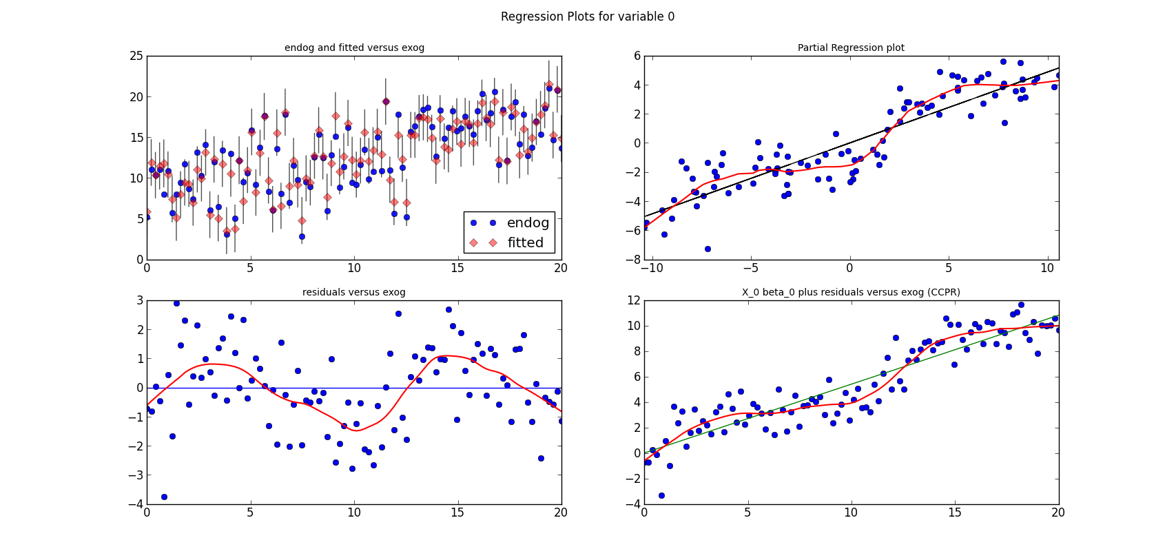
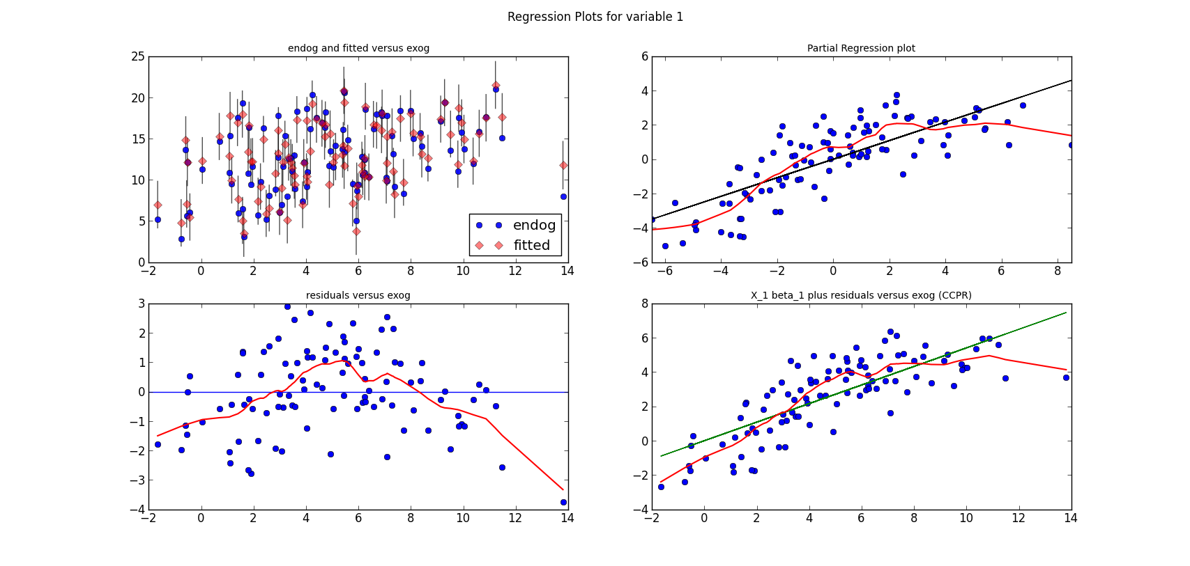
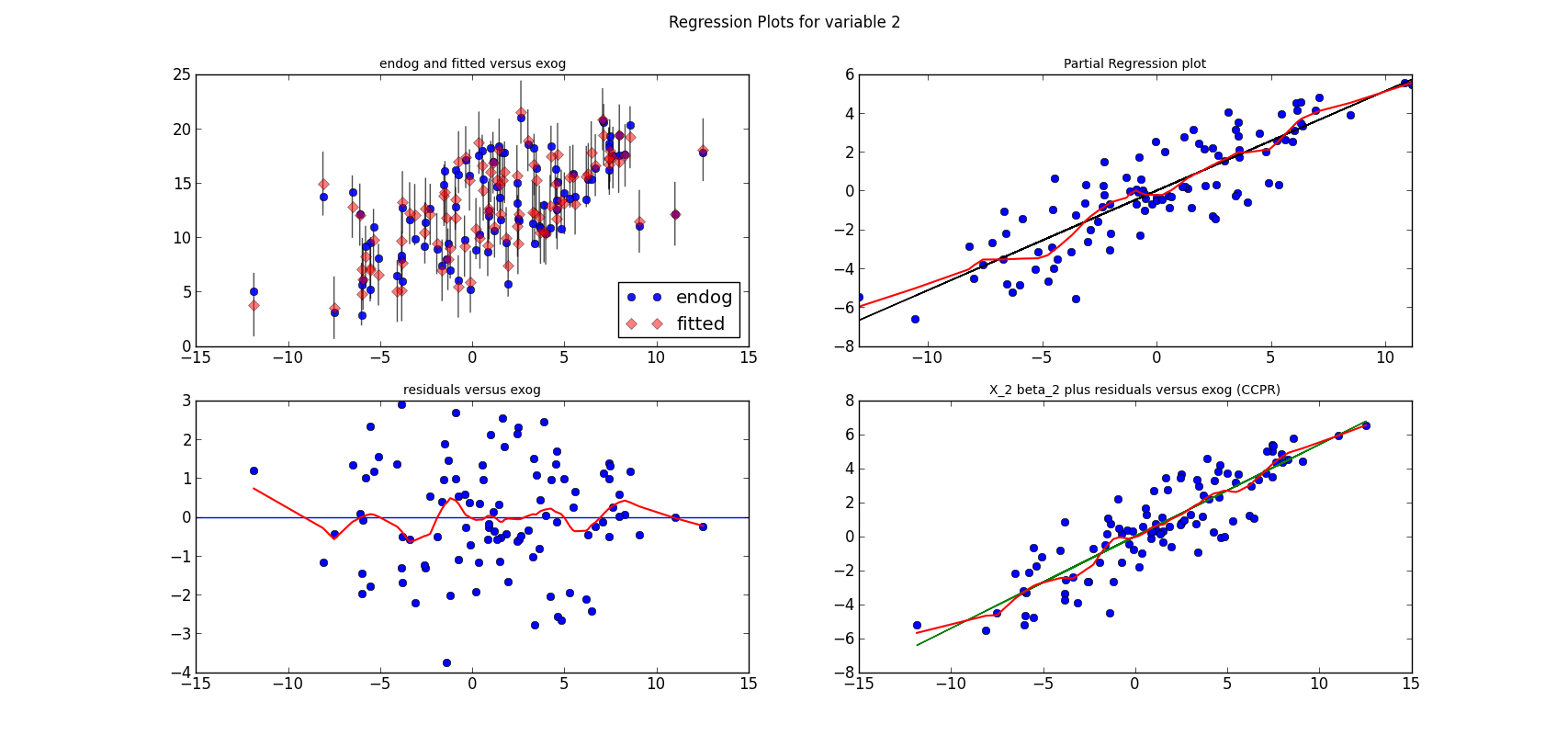
For now, just a question: Can you spot the mis-specification of the model?

I simulate a model, run a linear regression on three variables and a constant. Here is the estimation summary, which looks quite good, large R-squared, all variables significant, no obvious problems:
>>> print res.summary()
                                                        OLS Regression Results
==============================================================================
Dep. Variable:                      y   R-squared:                       0.901
Model:                            OLS   Adj. R-squared:                  0.898
Method:                 Least Squares   F-statistic:                     290.3
Date:                Thu, 10 May 2012   Prob (F-statistic):           5.31e-48
Time:                        13:15:22   Log-Likelihood:                -173.85
No. Observations:                 100   AIC:                             355.7
Df Residuals:                      96   BIC:                             366.1
Df Model:                           3
==============================================================================
                 coef    std err          t      P>|t|      [95.0% Conf. Int.]
------------------------------------------------------------------------------
x1             0.4872      0.024     20.076      0.000         0.439     0.535
x2             0.5408      0.045     12.067      0.000         0.452     0.630
x3             0.5136      0.030     16.943      0.000         0.453     0.574
const          4.6294      0.372     12.446      0.000         3.891     5.368
==============================================================================
Omnibus:                        0.945   Durbin-Watson:                   1.570
Prob(Omnibus):                  0.624   Jarque-Bera (JB):                1.031
Skew:                          -0.159   Prob(JB):                        0.597
Kurtosis:                       2.617   Cond. No.                         33.2
==============================================================================
The following three graphs are refactored versions of the regression plots. Each graph looks at the data and estimation results with respect to one of the three variables. (The graphs look better in original size.)
The short lines in the first subplot of each graph are the prediction confidence intervals for each observation.
The code is short, if we have the (still unpublished) helper functions.
res is an OLS results instance
from regressionplots_new import plot_regress_exog

fig9 = plot_regress_exog(res, exog_idx=0)
add_lowess(fig9, ax_idx=1, lines_idx=0)
add_lowess(fig9, ax_idx=2, lines_idx=0)
add_lowess(fig9, ax_idx=3, lines_idx=0)

fig10 = plot_regress_exog(res, exog_idx=1)
add_lowess(fig10, ax_idx=1, lines_idx=0)
add_lowess(fig10, ax_idx=2, lines_idx=0)
add_lowess(fig10, ax_idx=3, lines_idx=0)

fig11 = plot_regress_exog(res, exog_idx=2)
add_lowess(fig11, ax_idx=1, lines_idx=0)
add_lowess(fig11, ax_idx=2, lines_idx=0)
add_lowess(fig11, ax_idx=3, lines_idx=0)

Tuesday, May 8, 2012

Plots in statsmodels: qqplot

Other news first, since I haven't managed to catch up with the blogs:
  • statsmodels has four students in GSoC, the first four projects described in my previous post. Congratulations to Alexandre, Divyanshu, George and Justin
  • statsmodels 0.4.0 has been release with new name without scikits in front, more on pypi
statsmodels has a graphics subdirectory, where we started to collect some of the common statistical plots. To make the documentation a bit more exciting, I am adding plots directly to the docstrings for the individual functions. Currently, we don't have many of them in the online documentation yet, two examples violin_plot and bean_plot.
A note on the documentation: Skipper improved the frontpage, which makes it easier to find the documentation for the latest released version and for the development version. Currently, the development version is better and is improving, and it is incompatible with the 0.4.0 release in only one part.

quantile-quantile plot: qqplot

The documentation for the function is here. The function signature is
qqplot(data, dist=stats.norm, distargs=(), a=0, loc=0, scale=1, fit=False, line=False, ax=None)
I am not copying the entire docstring, what I would like to present here are some examples and how to work with the plots.
The first example is from the docstring. I don't like the default, so I kept adding keyword arguments until the plot is more to my taste.
  • The first plot uses no keywords and assumes normal distribution, and does not standardize the data.
  • The second plot adds line='s', which according to the docstring
    's' - standardized line, the expected order statistics are scaled
          by the standard deviation of the given sample and have the mean
          added to them
    
    corresponds to the line after fitting location and scale for the normal distribution
  • The third plot adds fit=True to get standardized sample quantiles and plots the 45 degree line. That's the plot I would prefer.
  • The fourth plot is similar to the third plot, but with the t distribution instead of the normal distribution. I was surprised that the third and fourth plot look the same, until I checked and it turned out that the fitted t distribution has a huge degrees of freedom parameter and so is essentially identical to the normal distribution.


I will go over the code to produce this below.
I started the second example to see whether fitting the t distribution works correctly. Instead of using real data, I generate 1000 observations with a t distribution with df=4 and standard location(0) and scale (1).
  • The first plot fits a normal distribution, keywords: line='45', fit=True
  • The second plot fits the t distribution, keywords: dist=stats.t, line='45', fit=True
  • The third plot is the same as the second plot, but I fit the t distribution myself, instead of having qqplot do it. keywords: dist=stats.t, distargs=(dof,), loc=loc, scale=scale, line='45'. I added the estimated parameters into a text insert in the plot. qqplot currently doesn't tell us what the fitted parameters are.


The Code

Here was my first attempt, following the docstring example
from scipy import stats
import statsmodels.api as sm

#estimate to get the residuals
data = sm.datasets.longley.load()
data.exog = sm.add_constant(data.exog)
mod_fit = sm.OLS(data.endog, data.exog).fit()
res = mod_fit.resid

fig = sm.graphics.qqplot(res, dist=stats.t, line='45', fit=True)
fig.show()
It works but the x-axis goes from -3 to 3, while there are only values from -2 to 2.
Detour to some background
A while ago we had a discussion on the mailing list what a plot in statsmodels should return. With the helpful comments of John Hunter, we finally agreed that plots should take an ax (matplotlib axis) argument if it's meaningful, and always return a figure instance fig. If ax is None, or the plot is a combination plot (several plots in one figure), then a figure is created and returned. If ax is given, then that is used to attach the plot elements. Ralf Gommers converted our plot functions to follow this pattern, besides that, he also wrote several of the plots that are currently in statsmodels.
So, to change the axis limits in the above graph, all I have to add is:
fig.axes[0].set_xlim(-2, 2)
The resulting plot is then the same as the third plot in the first graph above.
The first graph
Here is now the script for the first graph in several stages:
First I import some modules and calculate the residuals following the example
from scipy import stats
from matplotlib import pyplot as plt
import statsmodels.api as sm

#example from docstring
data = sm.datasets.longley.load()
data.exog = sm.add_constant(data.exog)
mod_fit = sm.OLS(data.endog, data.exog).fit()
res = mod_fit.resid
Then I hardcode a left position for text inserts, and create a matplotlib figure instance
left = -1.8
fig = plt.figure()
Next we can add the first subplot. The only keyword arguments for qqplot is ax to tell qqplot to attach the plot to my first subplot. Since I want to insert a text to describe the keywords, I needed to spend some time with the matplotlib documentation. As we have a reference to the axis instance, it is easy to change or add plot elements
ax = fig.add_subplot(2, 2, 1)
sm.graphics.qqplot(res, ax=ax)
top = ax.get_ylim()[1] * 0.75
txt = ax.text(left, top, 'no keywords', verticalalignment='top')
txt.set_bbox(dict(facecolor='k', alpha=0.1))
The other subplots follow the same pattern. I didn't try to generalize or avoid hardcoding
ax = fig.add_subplot(2, 2, 2)
sm.graphics.qqplot(res, line='s', ax=ax)
top = ax.get_ylim()[1] * 0.75
txt = ax.text(left, top, "line='s'", verticalalignment='top')
txt.set_bbox(dict(facecolor='k', alpha=0.1))

ax = fig.add_subplot(2, 2, 3)
sm.graphics.qqplot(res, line='45', fit=True, ax=ax)
ax.set_xlim(-2, 2)
top = ax.get_ylim()[1] * 0.75
txt = ax.text(left, top, "line='45', \nfit=True", verticalalignment='top')
txt.set_bbox(dict(facecolor='k', alpha=0.1))

ax = fig.add_subplot(2, 2, 4)
sm.graphics.qqplot(res, dist=stats.t, line='45', fit=True, ax=ax)
ax.set_xlim(-2, 2)
top = ax.get_ylim()[1] * 0.75
txt = ax.text(left, top, "dist=stats.t, \nline='45', \nfit=True",
              verticalalignment='top')
txt.set_bbox(dict(facecolor='k', alpha=0.1))
The final step is to adjust the layout, so that axis labels don't overlap with other subplots if the graph is not very large
fig.tight_layout()
The second graph
The second graph follows the same pattern with a few changes.
First we generate a random sample using scipy.stats which under the hood uses the random numbers from numpy. You can notice here that I am cheating. I ran the script several times to find "nice" seeds. Especially in smaller samples, qqplot might often not be very good in distinguishing normal and t distributions.
import numpy as np
seed = np.random.randint(1000000)
print 'seed', seed
seed = 461970  #nice seed for nobs=1000
#seed = 571478  #nice seed for nobs=100
#seed = 247819  #for nobs=100, estimated t is essentially normal
np.random.seed(seed)
rvs = stats.t.rvs(4, size=1000)
The first two subplot are very similar to what is in the first graph
fig2 = plt.figure()
ax = fig2.add_subplot(2, 2, 1)
fig2 = sm.graphics.qqplot(rvs, dist=stats.norm, line='45', fit=True, ax=ax)
top = ax.get_ylim()[1] * 0.75
xlim = ax.get_xlim()
frac = 0.1
left = xlim[0] * (1-frac) + xlim[1] * frac
txt = ax.text(left, top, "normal", verticalalignment='top')
txt.set_bbox(dict(facecolor='k', alpha=0.1))

ax = fig2.add_subplot(2, 2, 2)
fig2 = sm.graphics.qqplot(rvs, dist=stats.t, line='45', fit=True, ax=ax)
top = ax.get_ylim()[1] * 0.75
xlim = ax.get_xlim()
frac = 0.1
left = xlim[0] * (1-frac) + xlim[1] * frac
txt = ax.text(left, top, "t", verticalalignment='top')
txt.set_bbox(dict(facecolor='k', alpha=0.1))
For the third plot, I estimate the parameters of the t-distribution to see whether I get the same results as in the second plot (I do), and so I can insert the parameter estimates into the plot
params = stats.t.fit(rvs)
dof, loc, scale = params
ax = fig2.add_subplot(2, 2, 4)
fig2 = sm.graphics.qqplot(rvs, dist=stats.t, distargs=(dof,), loc=loc,
                 scale=scale, line='45', fit=False, ax=ax)
top = ax.get_ylim()[1] * 0.75
xlim = ax.get_xlim()
frac = 0.1
left = xlim[0] * (1-frac) + xlim[1] * frac
txt = ax.text(left, top, "t \ndof=%3.2F \nloc=%3.2F, \nscale=%3.2F" % tuple(params),
              verticalalignment='top')
txt.set_bbox(dict(facecolor='k', alpha=0.1))
That's it for the plots, now I need to add them to the statsmodels documentation.

PS: normality tests, details left for another day

qqplots give us a visual check whether a sample follows a specific distribution. The case that we are interested in most often, is a test for normality. Scipy.stats and statsmodels have several normality tests. The ones I have written recently are Anderson-Darling and Lillifors. Lillifors is a Kolmogorov-Smirnov test for normality when mean and variance are estimated. Calculating a statistical test provides a more reliable test than a "vague" visual inspection, but these tests do not point us to a specific alternative and provide less information about the direction in which a null hypothesis might be incorrect.
Using the residuals in the first example, neither test rejects the Null Hypothesis that the residuals come from a normal distribution
>>> normal_ad(res)
(0.43982328207860633, 0.25498161947268855)
>>> lillifors(res)
(0.17229856392873188, 0.2354638181341876)
On the other hand, in the second example with 1000 observations from the t distribution, the assumption that the data comes from a normal distribution is clearly rejected
>>> normal_ad(rvs)
(6.5408483355136013, 4.7694160497092537e-16)
>>> lillifors(rvs)
(0.05919821253474411, 8.5872265678140885e-09)
PPS:
I'm reluctant to publish the import path, because I had forgotten to add them to a proper place for 0.4.0, and the import location will not stay where it is. It took me a few minutes to find out that they are not on any recommended import path when I wrote these scripts
>>> from statsmodels.stats.adnorm import normal_ad
>>> from statsmodels.stats.lilliefors import lillifors

Wednesday, April 11, 2012

Statsmodels and Google Summer of Code 2012

I didn't have much time or motivation to work on my blog these last weeks, mainly because I was busy discussing Google Summer of Code and preparing a new release for statsmodels.

So here is just an update on our Google Summer of Code candidates and their projects. This year was a successful year in attracting student proposals. We have six proposals, five of them we discussed quite extensively on our mailing list before the application.

Of the five projects, the first two are must-haves for econometrics or statistical packages, one on System of Equations, the other on Nonlinear Least-Squares and Nonlinear Robust Models. The next two are nonparametric or semi-parametric methods, one more traditional kernel estimation, the other using Empirical Likelihood which is a relatively new approach that has become popular in recent research both in econometrics and in statistics. The fifth is on Dynamic Linear Models mainly using Kalman filter and a Bayesian approach, which would extend the depth of statsmodels in time series analysis.

All topics would be valuable extensions to statsmodels and significantly increase our coverage of statistics and econometrics. From the discussion on the mailing list I think that all candidates are qualified to bring the projects to a successful finish.

Estimating System of Equations

This is a standard econometrics topic, but I only recently found that graphical models and causal models discussed in other fields have a large overlap with this. In the case of a system of simultaneous equations, we have several variables that depend on each other. The simplest case in economics is a market equilibrium, where the demanded and supplied quantities depend on the price, and the price depends on the supply and demand. The estimation methods commonly used in this area are two-stage and three-stage least-squares and limited and full information maximum likelihood estimation. The first part of the project starts with the simpler case when we have several response variables, but they don't depend on each other simultaneously, although they can depend on past values of other response variables. I'm very glad that someone is picking this one up.

Extension of Linear to Non Linear Models

This project has two parts, the first is extending the linear least-squares model to the non-linear case, the second part is to implement non-linear models for robust estimation. Non-linear least squares is available in scipy for example with scipy.optimize.curve_fit. However, in the statsmodels version we want to provide all the usual results statistics and statistical tests. The second part will implement two robust estimators for non-linear model, that have been shown to be most successful in recent Monte Carlo studies comparing different robust estimators for non-linear equations. Robust estimation here refers to the case when there are possibly many outliers in the data. My guess is that these will become the most used models of all proposals.

Nonparametric Estimation

This project extends the kernel based method in statsmodels from the univariate to the multivariate case, will provide better bandwidth selection, and then implement nonparametric function estimation. Multivariate kernel density estimation should complement scipy.stats.gaussian_kde which only works well with distributions that are approximately normal shaped or have only a single peak. Another extension is to provide kernels and estimation methods for discrete variables. These methods have been on our wishlist for a while, but only the univariate case has been included in statsmodels so far.

Empirical Likelihood

This is a relatively new approach in statistics and econometrics that avoids the distributional assumptions in estimation and in statistical tests. Instead of relying on a known distribution in small samples, where we often assume normal distribution, or instead of relying on the asymptotic normal distribution in large samples, this approach estimates the distribution in a nonparametric way. This is similar, to some extend, to the difference between, for example, a t-test and a rank-based Mann–Whitney U or Wilcoxon test, which are available in scipy.stats. The advantages are that in smaller samples the estimates and tests are more accurate when the distribution is not known, and in many cases, for example in finance, most tests show that the assumption of normal distribution does not hold. For this project, I still have to catch up with some readings because I'm only familiar with a small part of this literature, mainly on empirical likelihood in relation to Generalized Method of Moments (GMM).

Dynamic Linear Models

This covers statespace models implemented by Kalman Filter for multivariate time series models, both from a likelihood and a Bayesian perspective. The project expands the coverage of statsmodels in linear time series analysis, the first area where we get a good coverage of models. Currently, we have univariate AR and ARIMA, vector autoregressive models VAR, and structural VAR. Part of this project would be to get a good cython based implementation of Kalman filters. Wes has started a libray, statlib, for this last year, however, it is still incomplete and needs to be integrated with statsmodels. Another advantage of this project is that it increases our infrastructure and models for macro-econometrics, estimation of macroeconomic models and dynamic stochastic general equilibrium DSGE models, which is currently still Matlab dominated, as far as I can tell.

Now we still have to see how many GSoC slots we will get, but we have the chance this year to get a large increase in the speed of development of statsmodels, and we can reduce the number of cases where someone needs to run to R, or Stata, or Matlab because there is no implementation for a statistical analysis available in Python.

Sunday, March 4, 2012

Numerical Accuracy in Linear Least Squares and Rescaling

The Problem

(Warning upfront: there are problems to replicate this, more below)

A week ago, I stumbled on this Numerical_Comparison_of_Statistical_Software which presents some test results for numerical accuracy of statistical packages.

For linear regression, there is one test, Longley, that we have in the datasets in statsmodels. But I wanted to look at Filip which sounds like a difficult case, neither SAS nor SPSS produced a solution. Let's see how badly statsmodels and numpy are doing, or maybe not.

The model is a polynomial of degree 10. Description, data, certified values and a plot are on the NIST website here

1 Predictor Variable
82 Observations
Higher Level of Difficulty
Model: Polynomial, 11 Parameters

I parsed the data into an array dta, first column is the endogeous, y, variable second column is the exogenous, x, variable. I saved y in endog. I also parsed the main NIST result in params_nist, first column parameters, second column their standard deviation.

Fitting a Polynomial

Since it is a polynomial problem, let us treat it as such and use the polynomials from numpy.

First try, use the old polyfit function

>>> p_params = np.polyfit(dta[:,1], endog, 10)[::-1]
>>> p_params
array([-1467.48963361, -2772.17962811, -2316.37111156, -1127.97395547,
        -354.47823824,   -75.1242027 ,   -10.87531817,    -1.062215  ,
          -0.06701912,    -0.00246781,    -0.0000403 ])
>>> log_relative_error(p_params, params_nist[:,0])
array([ 7.87929761,  7.88443445,  7.88840683,  7.89138269,  7.89325784,
        7.89395336,  7.89341841,  7.89162977,  7.88859034,  7.88432427,
        7.87887292])

Not bad, following the description on the Wikipedia page, I wrote a function log_relative_error that tells us how many significant digits agreement is between the two arrays. polyfit agrees at 7 to 8 significant digits, that's about the same as S-Plus on the Wikipedia page.

Let's work properly with polynomials and use the new polynomial package in numpy. Charles Harris wrote it and is still expanding and improving it.

>>> poly = np.polynomial.Polynomial.fit(dta[:,1],endog, 10)
>>> poly
Polynomial([ 0.88784146,  0.10879327, -0.53636698,  0.28747072,  2.20567367,
       -1.31072158, -4.21841581,  1.76229897,  3.8096025 , -0.77251557,
       -1.30327368], [-8.78146449, -3.13200249])

Oops, these numbers don't look like the NIST numbers. The last numbers, [-8.78146449, -3.13200249], show the domain of the polynomial, our values have been transformed. A bit of introspection, and we figure out how to change the domain. To get the "standard" representation, we can transform the domain back to the standard domain (-1, 1).

>>> poly.convert(domain=(-1,1))
Polynomial([-1467.48961423, -2772.17959193, -2316.37108161, -1127.97394098,
        -354.4782337 ,   -75.12420174,   -10.87531804,    -1.06221499,
          -0.06701912,    -0.00246781,    -0.0000403 ], [-1.,  1.])

Now, this looks more like NIST, it even agrees at 13 to 14 significant digits

>>> log_relative_error(poly.convert(domain=(-1,1)).coef, params_nist[:,0])
array([ 13.72347502,  13.84056851,  13.81494335,  13.70878715,
        13.78207216,  13.79374075,  13.6729684 ,  13.71128925,
        13.75445952,  13.68695573,  13.67736436])

Nice job Charles. No problem fitting this polynomial with numpy.

Linear Regression

In the previous part we knew we were fitting a polynomial, but lets treat it just as a standard linear regression problem and use scikits.statsmodels.

First try: just create the design matrix in the simplest way and estimate

>>> exog0 = dta[:,1:]**np.arange(11)
>>> res0 = sm.OLS(endog, exog0).fit()
>>> res0.params
array([ 8.443046917097718,  1.364996059973237, -5.350750046084954,
       -3.34190287892045 , -0.406458629495091,  0.257727311296307,
        0.119771653524165,  0.023140891929892,  0.002403995206457,
        0.000131618839544,  0.000002990001222])
>>> log_relative_error(res0.params, params_nist[:,0])
array([-0.002491507096328, -0.000213790029725,  0.00100436814061 ,
        0.001288615104161,  0.000498264786078, -0.00148737673275 ,
       -0.004756810105056, -0.009359738327099, -0.015305377783833,
       -0.022566206229652, -0.031085341541384])

Bummer, 0 significant digits, way off.

We can print the full summary of the results, maybe we see something

>>> print res0.summary()
                            OLS Regression Results
==============================================================================
Dep. Variable:                      y   R-squared:                       0.996
Model:                            OLS   Adj. R-squared:                  0.995
Method:                 Least Squares   F-statistic:                     2390.
Date:                Sat, 03 Mar 2012   Prob (F-statistic):           1.85e-84
Time:                        23:47:45   Log-Likelihood:                 344.73
No. Observations:                  82   AIC:                            -673.5
Df Residuals:                      74   BIC:                            -654.2
Df Model:                           7
==============================================================================
                 coef    std err          t      P>|t|      [95.0% Conf. Int.]
------------------------------------------------------------------------------
const          8.4430     12.864      0.656      0.514       -17.189    34.075
x1             1.3650      6.496      0.210      0.834       -11.578    14.308
x2            -5.3508      9.347     -0.572      0.569       -23.974    13.273
x3            -3.3419     11.702     -0.286      0.776       -26.659    19.975
x4            -0.4065      5.923     -0.069      0.945       -12.209    11.396
x5             0.2577      1.734      0.149      0.882        -3.197     3.712
x6             0.1198      0.321      0.373      0.710        -0.520     0.759
x7             0.0231      0.038      0.604      0.548        -0.053     0.099
x8             0.0024      0.003      0.838      0.405        -0.003     0.008
x9             0.0001      0.000      1.072      0.287        -0.000     0.000
x10          2.99e-06   2.29e-06      1.303      0.197     -1.58e-06  7.56e-06
==============================================================================
Omnibus:                        1.604   Durbin-Watson:                   1.627
Prob(Omnibus):                  0.449   Jarque-Bera (JB):                1.379
Skew:                          -0.317   Prob(JB):                        0.502
Kurtosis:                       2.961   Cond. No.                        -1.#J
==============================================================================

The smallest eigenvalue is  -0.38. This might indicate that there are
strong multicollinearity problems or that the design matrix is singular.

R square is 0.996, so we are fitting the curve pretty well, but our design matrix with the polynomial is not positive definite. There is even a negative eigenvalue. A negative eigenvalue sounds strange, a quadratic form shouldn't have them. Just to make sure that this is not a bug, check with numpy

>>> np.linalg.eigvalsh(np.dot(exog0.T, exog0)).min()
-0.38006444279775781
>>> np.linalg.eigvals(np.dot(exog0.T, exog0)).min()
-0.00011161167956978682

I'm still suspicious, but I delay the detour into numpy's and scipy's linalg modules.

One more check of our regression results, the residual standard error is not very far away from the Nist numbers:

>>> np.sqrt(res0.mse_resid), 0.334801051324544E-02,
(0.0038044343586352601, 0.0033480105132454399)

Conclusion: If you try to fit a linear regression with a non-positive definite design matrix, then the parameters are not identified, but we can still get a good fit.

(Technical aside: statsmodels uses by default the generalized inverse, pinv, for linear regression. So it just drops the eigenvalues below a threshold close to zero. The parameter estimates will be closer to a penalized Ridge regression. But don't quote me on the last part since I don't remember where I read that pinv is the limit of a Ridge problem.)

The question for statsmodels is what to do about it.

One solution that works in this case, as we have seen with numpy polynomials, is to rescale the explanatory variables or design matrix. I'm showing one example below. My working title for this post was: Don't do this, or do we have to do it for you? Is it the responsibility of the user not to use a design matrix that numerically doesn't make much sense and we can only warn, or should we automatically transform the design matrix to make it numerically more stable. The latter will be costly and might not be required in 99% of the cases?

Another issue is that there are many different ways to do the linear algebra, and we have not investigated much what might work better or worse in different cases. See Addendum below for the effect that linear algebra can have in numerically unstable problems.

Rescaling the Design Matrix

Our design matrix looks pretty bad, variables vary in a large range and the correlation is very high

>>> np.set_printoptions(precision=3)
>>> print np.max(np.abs(exog0),0)
[  1.000e+00   8.781e+00   7.711e+01   6.772e+02   5.947e+03   5.222e+04
   4.586e+05   4.027e+06   3.536e+07   3.105e+08   2.727e+09]
>>> print np.corrcoef(exog0[:,1:], rowvar=0)
[[ 1.    -0.991  0.969 -0.938  0.904 -0.87   0.838 -0.808  0.782 -0.758]
 [-0.991  1.    -0.993  0.975 -0.951  0.925 -0.899  0.874 -0.851  0.83 ]
 [ 0.969 -0.993  1.    -0.994  0.981 -0.963  0.943 -0.924  0.904 -0.886]
 [-0.938  0.975 -0.994  1.    -0.996  0.986 -0.973  0.958 -0.943  0.928]
 [ 0.904 -0.951  0.981 -0.996  1.    -0.997  0.99  -0.98   0.968 -0.957]
 [-0.87   0.925 -0.963  0.986 -0.997  1.    -0.998  0.992 -0.985  0.976]
 [ 0.838 -0.899  0.943 -0.973  0.99  -0.998  1.    -0.998  0.994 -0.988]
 [-0.808  0.874 -0.924  0.958 -0.98   0.992 -0.998  1.    -0.999  0.995]
 [ 0.782 -0.851  0.904 -0.943  0.968 -0.985  0.994 -0.999  1.    -0.999]
 [-0.758  0.83  -0.886  0.928 -0.957  0.976 -0.988  0.995 -0.999  1.   ]]

Now we can use just the simplest transform, limit the maximum absolute value to be one:

exog1 = exog0 / np.max(np.abs(exog0),0)

After running the regression on the rescaled design matrix, we see an agreement with the NIST benchmark results at around 7 to 8 significant digits both for the parameters and for the standard deviation of the parameter estimates, bse in statsmodels:

>>> res1 = sm.OLS(endog, exog1).fit()
>>> params_rescaled = res1.params / np.max(np.abs(exog0), 0)
>>> log_relative_error(params_rescaled, params_nist[:,0])
array([ 7.419,  7.414,  7.409,  7.402,  7.394,  7.384,  7.373,  7.36 ,
        7.346,  7.331,  7.314])
>>> bse_rescaled = res1.bse / np.max(np.abs(exog0),0)
>>> log_relative_error(bse_rescaled, params_nist[:,1])
array([ 8.512,  8.435,  8.368,  8.308,  8.255,  8.207,  8.164,  8.124,
        8.089,  8.057,  8.028])

Also R squared and the standard deviation of the residuals (using appropriate degrees of freedom) agrees with the NIST numbers at around 10 and 7 digits, resp.

>>> log_relative_error(res1.rsquared, 0.996727416185620)
10.040156510920081

>>> log_relative_error(np.sqrt(res1.mse_resid), 0.334801051324544E-02)
7.8575015681097371

So we are doing pretty well just with a simple rescaling of the variables. Although, the comment at the end of print res1.summary() still reports a smallest eigenvalue of -1.51e-15, so essentially zero. But I worry about this later. I looked initially at another way of rescaling the design matrix but didn't check yet how the choice of the rescaling will affect the results

Addendum 1: Smallest eigenvalue of ill-conditioned array

Going back to the original design matrix without rescaling, define the moment matrix X'X:

>>> xpx0 = np.dot(exog0.T, exog0)

the eigenvalues, assuming a symmetric matrix, are

>>> np.sort(np.linalg.eigvalsh(xpx0))
array([ -3.79709e-01,   1.14869e-05,   4.40507e-03,   3.20670e+00,
         7.91804e+02,   1.05833e+03,   3.98410e+05,   2.31485e+08,
         4.28415e+11,   1.93733e+15,   5.17955e+19])

This looks very badly conditioned. the largest eigenvalue is 5e19, the smallest is "around zero".

We can compare different algorithms to calculate the smallest eigenvalues (splinalg is scipy.linalg)

>>> np.sort(np.linalg.eigvals(xpx0))[:4]
array([  3.41128e-04,   5.58946e-04,   1.23213e-02,   3.33365e+00])
>>> np.sort(splinalg.eigvalsh(xpx0))[:4]
array([ -2.14363e+03,  -2.00323e-01,   1.26094e-05,   4.40956e-03])
>>> np.sort(splinalg.eigvals(xpx0))[:4]
array([ -3.66973e-05+0.j,   1.61750e-04+0.j,   7.90465e-03+0.j,
         2.01592e+00+0.j])

>>> np.sort(np.linalg.svd(xpx0)[1])[:4]
array([  2.84057e-05,   4.91555e-04,   7.28252e-03,   3.41739e+00])
>>> np.sort(splinalg.svd(xpx0)[1])[:4]
array([  2.19202e-05,   7.11920e-04,   7.00790e-03,   3.28229e+00])

>>> np.sort(np.linalg.svd(exog0)[1]**2)[:4]
array([  1.65709e-11,   3.08225e-08,   2.48138e-05,   1.08036e-02])
>>> np.sort(splinalg.svd(exog0)[1]**2)[:4]
array([  1.65708e-11,   3.08225e-08,   2.48138e-05,   1.08036e-02])

So, we see that they are pretty much all over the place, from -0.38 to 2.8e-05. The last version with singular value decomposition is the closest to what statsmodels uses with pinv. It also looks like I picked the worst algorithm for the regression summary in this case.

Warning: Calculations at machine precision are not necessarily deterministic, in the sense that if you run it repeatedly you might not always get the same results. There are several cases on the scipy and numpy mailing lists that report that the results might "randomly" switch between several patterns. And the results won't agree on different operating systems, compilers and versions of the linear algebra libraries. So, I don't expect that these results can be replicated in exactly the same way.

Addendum 2: scipy.linalg versus numpy.linalg

To avoid getting these changing results whenever I re-ran the script while preparing this post, I changed the statsmodels source to use scipy.linalg.pinv instead of numpy.linalg.pinv. I expected more replicable results, however what I found is:

>>> exog0 = dta[:,1:]**np.arange(11)
>>> res0 = sm.OLS(endog, exog0).fit()
>>> log_relative_error(res0.params, params_nist[:,0])
array([ 5.31146488,  5.7400516 ,  6.53794562,  6.81318335,  6.81855769,
        7.22333339,  8.13319742,  7.38788711,  7.24457806,  7.18580677,
        7.12494176])
>>> log_relative_error(res0.bse, params_nist[:,1])
array([ 2.25861611,  2.25837872,  2.25825903,  2.25822427,  2.2582245 ,
        2.25823174,  2.25823693,  2.25823946,  2.25824058,  2.25824108,
        2.25824165])

Just by changing the algorithm that calculates the generalized inverse, I get agreement with the NIST data at 5 to 7 significant digits for the parameters and 2 digits for the standard error of the parameter estimates even with the very ill-conditioned original design matrix. That doesn't look so bad, much better than when using the numpy.linalg version.

(But I need to write proper tests and look at this when I can trust the results. I now have two python sessions open, one that imported the original source, and one that imported the source after changing the statsmodels source. Also, if I run this regression repeatedly the numbers changed once, but remained within the same neighborhood. Besides different algorithm there is also rcond which defines the cutoff in pinv. I didn't check whether that differs in the numpy and scipy versions.)

Conclusions

I think this test case on the NIST site is very well "cooked" to test the numerical accuracy of a linear regression program. The main lesson is that we shouldn't throw a numerically awful problem at a statistical package, unless we know that the package takes care for us of the basic tricks for making the problem numerically more stable. It's safer to make sure our design matrix is numerically sound.

Also, if we just want to estimate a polynomial function, then use the information and use a specialized algorithm, or, even better, use an orthogonal polynomial basis instead of power polynomials.

What does it mean for statistical analysis?

That, I'm not so sure. Multicollinearity is a serious issue, and there a various approaches for dealing with it. But my attitude so far has been:

If you work with real data and run into numerical problems, it's not a problem with numerical accuracy but with your data, or with your model.

We should still use basic precautions like scaling our variables appropriately, but if we have high multicollinearity, then it mainly means that the model that we specified is asking for information that's not in the data. In certain directions the data is not informative enough to reliably identify some parameters. Given measurement errors, noise in the data and misspecification, there are many other parts to worry about before machine precision becomes important. For a related discussion see this thread on the statsmodels mailinglist.

I tried before to come up with a case where standardizing (zscoring) the design matrix helps in improving the precision of the estimates but I didn't manage. Whether I zscored or not, the results where essentially the same. Now, I have a test case to add to statsmodels. I am sceptical about automatic rescaling, but I started a while ago to look into how to make it easier for users to use predefined transforms in statsmodels, instead of having to code them from scratch.

I'm not an expert in numerical analysis and don't intend to become one, my "numerical incompetence" has improved only a bit since this although I know now a bit more linear algebra.

I put a script with the NIST case in this gist. I haven't yet copied over the parts from the interpreter sessions.

A final comment:

I don't like long interpreter sessions, I usually convert everything as fast as possible to a script. For this, I copied everything directly from the session. After cleaning up the original script a bit, I'm getting different numbers for the log relative error (LRE). I'm now using scipy.linalg.pinv inside statsmodels, and LRE is in this case a measure for the behavior at machine precision, and bounces anywhere between 5 and 8. This is a good result in that we can still get estimates with a reasonable precision, but it makes LRE unreliable for replicating the results. I will make a proper script and unittest later, so that I can be more certain about how much the numbers change and whether there isn't a bug somewhere in my "live" session.